19 Joins

19.1 Introduction

数据分析很少只涉及单个数据框。通常你会拥有多个数据框，并且必须通过连接（join）将它们合并起来，以回答你感兴趣的问题。本章将向你介绍两种重要的连接类型：

Mutating joins, 从另一个数据框的匹配观测中添加新变量到一个数据框。
Filtering joins, 根据观测是否与另一个数据框中的观测匹配，从一个数据框中筛选观测。

我们将首先讨论键——用于在连接中关联一对数据框的变量。然后通过检查 nycflights13 包中数据集的键来巩固理论，并利用这些知识开始连接数据框。接着我们将讨论连接的工作原理，重点关注它们对行的操作。最后，我们将讨论非等值连接——一类提供比默认相等关系更灵活的键匹配方式的连接。

19.1.1 Prerequisites

在本章中，我们将使用 dplyr 的连接函数来探索 nycflights13 中的五个相关数据集。

library(tidyverse)
library(nycflights13)

19.2 Keys

要理解连接，首先需要了解两个表如何通过各自内部的键对进行关联。在本节中，你将学习两种类型的键，并查看 nycflights13 包数据集中两种键的示例。你还将学习如何检查键是否有效，以及如果表缺少键该怎么办。

19.2.1 Primary and foreign keys

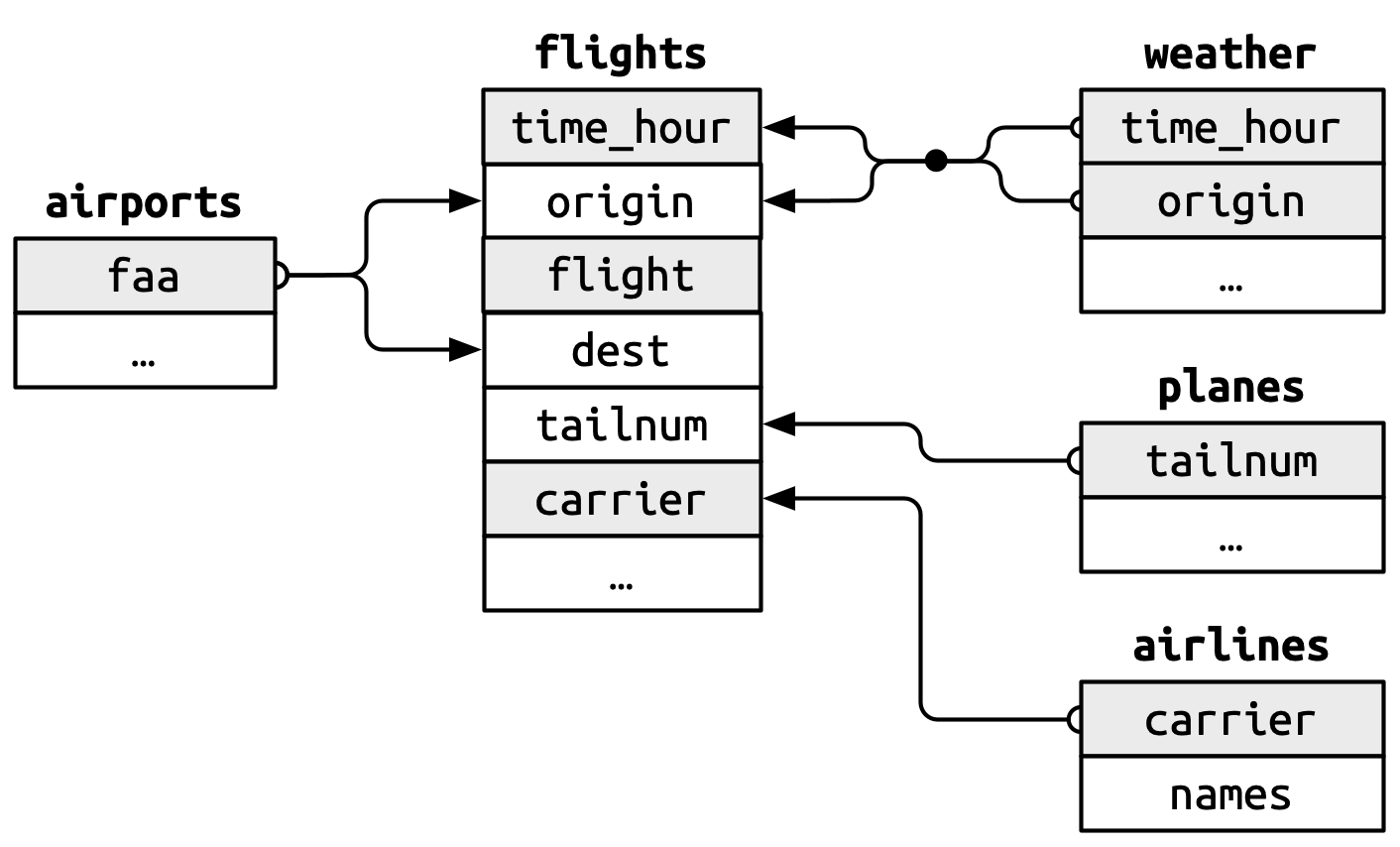
每次连接都涉及一对键：主键和外键。主键是唯一标识每个观测的一个变量或一组变量。当需要多个变量时，该键称为复合键。例如，在 nycflights13 中：

airlines 记录了每家航空公司的两条信息：其承运人代码和全称。你可以用其两个字母的承运人代码来识别航空公司，因此 carrier 是主键。

airlines
#> # A tibble: 16 × 2
#>   carrier name                    
#>   <chr>   <chr>                   
#> 1 9E      Endeavor Air Inc.       
#> 2 AA      American Airlines Inc.  
#> 3 AS      Alaska Airlines Inc.    
#> 4 B6      JetBlue Airways         
#> 5 DL      Delta Air Lines Inc.    
#> 6 EV      ExpressJet Airlines Inc.
#> # ℹ 10 more rows

airports 记录了每个机场的数据。你可以用其三个字母的机场代码来识别每个机场，因此 faa 是主键。

airports
#> # A tibble: 1,458 × 8
#>   faa   name                            lat   lon   alt    tz dst  
#>   <chr> <chr>                         <dbl> <dbl> <dbl> <dbl> <chr>
#> 1 04G   Lansdowne Airport              41.1 -80.6  1044    -5 A    
#> 2 06A   Moton Field Municipal Airport  32.5 -85.7   264    -6 A    
#> 3 06C   Schaumburg Regional            42.0 -88.1   801    -6 A    
#> 4 06N   Randall Airport                41.4 -74.4   523    -5 A    
#> 5 09J   Jekyll Island Airport          31.1 -81.4    11    -5 A    
#> 6 0A9   Elizabethton Municipal Airpo…  36.4 -82.2  1593    -5 A    
#> # ℹ 1,452 more rows
#> # ℹ 1 more variable: tzone <chr>

planes 记录了每架飞机的数据。你可以用其尾号来识别飞机，因此 tailnum 是主键。

planes
#> # A tibble: 3,322 × 9
#>   tailnum  year type              manufacturer    model     engines
#>   <chr>   <int> <chr>             <chr>           <chr>       <int>
#> 1 N10156   2004 Fixed wing multi… EMBRAER         EMB-145XR       2
#> 2 N102UW   1998 Fixed wing multi… AIRBUS INDUSTR… A320-214        2
#> 3 N103US   1999 Fixed wing multi… AIRBUS INDUSTR… A320-214        2
#> 4 N104UW   1999 Fixed wing multi… AIRBUS INDUSTR… A320-214        2
#> 5 N10575   2002 Fixed wing multi… EMBRAER         EMB-145LR       2
#> 6 N105UW   1999 Fixed wing multi… AIRBUS INDUSTR… A320-214        2
#> # ℹ 3,316 more rows
#> # ℹ 3 more variables: seats <int>, speed <int>, engine <chr>

weather 记录了起飞机场的天气数据。你可以通过地点和时间的组合来识别每个观测，因此 origin 和 time_hour 是复合主键。

weather
#> # A tibble: 26,115 × 15
#>   origin  year month   day  hour  temp  dewp humid wind_dir
#>   <chr>  <int> <int> <int> <int> <dbl> <dbl> <dbl>    <dbl>
#> 1 EWR     2013     1     1     1  39.0  26.1  59.4      270
#> 2 EWR     2013     1     1     2  39.0  27.0  61.6      250
#> 3 EWR     2013     1     1     3  39.0  28.0  64.4      240
#> 4 EWR     2013     1     1     4  39.9  28.0  62.2      250
#> 5 EWR     2013     1     1     5  39.0  28.0  64.4      260
#> 6 EWR     2013     1     1     6  37.9  28.0  67.2      240
#> # ℹ 26,109 more rows
#> # ℹ 6 more variables: wind_speed <dbl>, wind_gust <dbl>, …

外键是另一个表中与主键对应的变量（或一组变量）。例如：

flights$tailnum 是一个外键，对应主键 planes$tailnum.
flights$carrier 是一个外键，对应主键 airlines$carrier.
flights$origin 是一个外键，对应主键 airports$faa.
flights$dest 是一个外键，对应主键 airports$faa.
flights$origin-flights$time_hour 是一个复合外键，对应复合主键 weather$origin-weather$time_hour.

这些关系在 Figure 19.1 中进行了可视化总结。

The relationships between airports, planes, flights, weather, and airlines datasets from the nycflights13 package. airports$faa connected to the flights$origin and flights$dest. planes$tailnum is connected to the flights$tailnum. weather$time_hour and weather$origin are jointly connected to flights$time_hour and flights$origin. airlines$carrier is connected to flights$carrier. There are no direct connections between airports, planes, airlines, and weather data frames. — Figure 19.1: Connections between all five data frames in the nycflights13 package. Variables making up a primary key are colored grey, and are connected to their corresponding foreign keys with arrows.

你会注意到这些键设计中的一个优点：主键和外键几乎总是具有相同的名称，这（正如你稍后将看到的）将使连接操作更加简便。同样值得注意的是相反的关系：在多个表中使用的变量名几乎在每个地方都有相同的含义。只有一个例外：year 在 flights 中指出发年份，在 planes 中指制造年份。当我们真正开始连接表时，这一点将变得非常重要。

19.2.2 Checking primary keys

现在我们已经识别出每个表中的主键，最好验证它们是否确实能唯一标识每个观测。一种方法是使用 count() 对主键进行计数，并查找 n 大于 1 的记录。这表明 planes 和 weather 的主键情况良好：

planes |> 
  count(tailnum) |> 
  filter(n > 1)
#> # A tibble: 0 × 2
#> # ℹ 2 variables: tailnum <chr>, n <int>

weather |> 
  count(time_hour, origin) |> 
  filter(n > 1)
#> # A tibble: 0 × 3
#> # ℹ 3 variables: time_hour <dttm>, origin <chr>, n <int>

你还应检查主键中是否存在缺失值——如果某个值是缺失的，它就无法标识一个观测！

planes |> 
  filter(is.na(tailnum))
#> # A tibble: 0 × 9
#> # ℹ 9 variables: tailnum <chr>, year <int>, type <chr>, manufacturer <chr>,
#> #   model <chr>, engines <int>, seats <int>, speed <int>, engine <chr>

weather |> 
  filter(is.na(time_hour) | is.na(origin))
#> # A tibble: 0 × 15
#> # ℹ 15 variables: origin <chr>, year <int>, month <int>, day <int>,
#> #   hour <int>, temp <dbl>, dewp <dbl>, humid <dbl>, wind_dir <dbl>, …

19.2.3 Surrogate keys

到目前为止，我们还没有讨论 flights 的主键。这里它并不是特别重要，因为没有其他数据框将其用作外键，但考虑它仍然有用，因为如果我们有某种方式向他人描述观测，处理它们会更容易。

经过一些思考和试验，我们确定有三个变量共同唯一标识每个航班：

flights |> 
  count(time_hour, carrier, flight) |> 
  filter(n > 1)
#> # A tibble: 0 × 4
#> # ℹ 4 variables: time_hour <dttm>, carrier <chr>, flight <int>, n <int>

没有重复记录是否自动使 time_hour-carrier-flight 成为主键？这当然是个好的起点，但并不能保证。例如，海拔和纬度是 airports 的良好主键吗？

airports |>
  count(alt, lat) |> 
  filter(n > 1)
#> # A tibble: 1 × 3
#>     alt   lat     n
#>   <dbl> <dbl> <int>
#> 1    13  40.6     2

显然，通过海拔和纬度来标识机场是个糟糕的主意，而且通常仅从数据本身无法判断一组变量能否构成一个好的主键。但对于航班来说，time_hour, carrier 和 flight 的组合似乎是合理的，因为如果同一时间空中有多个相同航班号的航班，航空公司和乘客都会非常困惑。

也就是说，使用行号引入一个简单的数值代理键可能更好：

flights2 <- flights |> 
  mutate(id = row_number(), .before = 1)
flights2
#> # A tibble: 336,776 × 20
#>      id  year month   day dep_time sched_dep_time dep_delay arr_time
#>   <int> <int> <int> <int>    <int>          <int>     <dbl>    <int>
#> 1     1  2013     1     1      517            515         2      830
#> 2     2  2013     1     1      533            529         4      850
#> 3     3  2013     1     1      542            540         2      923
#> 4     4  2013     1     1      544            545        -1     1004
#> 5     5  2013     1     1      554            600        -6      812
#> 6     6  2013     1     1      554            558        -4      740
#> # ℹ 336,770 more rows
#> # ℹ 12 more variables: sched_arr_time <int>, arr_delay <dbl>, …

代理键在与他人沟通时特别有用：告诉某人查看航班 2001，比说查看 2013年1月3日上午9点起飞的 UA430 航班要容易得多。

19.2.4 Exercises

我们在 Figure 19.1 中忘记了绘制 weather 和 airports 之间的关系。它们的关系是什么？在图中应该如何表示？
weather 只包含纽约三个起飞机场的信息。如果它包含美国所有机场的天气记录，那么它会与 flights 建立什么额外的连接？
year, month, day, hour 和 origin 这些变量几乎构成了 weather 的复合键，但有一个小时存在重复观测。你能找出那个小时有什么特殊之处吗？
我们知道一年中有些特殊日子（例如平安夜和圣诞节）的乘客数量比平时少。你如何将这种数据表示为一个数据框？主键会是什么？它将如何与现有的数据框连接？
绘制一张图说明 Lahman 包中 Batting、People 和 Salaries 数据框之间的连接关系。再绘制另一张图展示 People, Managers, AwardsManagers 之间的关系。你如何描述 Batting, Pitching 和 Fielding 数据框之间的关系？

19.3 Basic joins

现在你已经理解了数据框如何通过键连接，我们可以开始使用连接来更好地理解 flights 数据集。 dplyr 提供了六个连接函数：left_join(), inner_join(), right_join(), full_join(), semi_join() 和 anti_join()。它们都有相同的接口：接收一对数据框（x 和 y）并返回一个数据框。输出中的行和列顺序主要由 x 决定。

在本节中，你将学习如何使用一个变异连接 left_join() 以及两个筛选连接 semi_join() 和 anti_join()。下一节你将详细了解这些函数的工作原理，以及剩余的 inner_join(), right_join() 和 full_join()。

19.3.1 Mutating joins

变异连接（mutating join）允许你合并两个数据框的变量：它首先通过键匹配观测，然后将变量从一个数据框复制到另一个。与 mutate() 类似，连接函数会将变量添加到右侧，因此如果你的数据集有很多变量，你可能看不到新增的变量。为了示例清晰，我们将创建一个仅包含六个变量的简化数据集¹：

flights2 <- flights |> 
  select(year, time_hour, origin, dest, tailnum, carrier)
flights2
#> # A tibble: 336,776 × 6
#>    year time_hour           origin dest  tailnum carrier
#>   <int> <dttm>              <chr>  <chr> <chr>   <chr>  
#> 1  2013 2013-01-01 05:00:00 EWR    IAH   N14228  UA     
#> 2  2013 2013-01-01 05:00:00 LGA    IAH   N24211  UA     
#> 3  2013 2013-01-01 05:00:00 JFK    MIA   N619AA  AA     
#> 4  2013 2013-01-01 05:00:00 JFK    BQN   N804JB  B6     
#> 5  2013 2013-01-01 06:00:00 LGA    ATL   N668DN  DL     
#> 6  2013 2013-01-01 05:00:00 EWR    ORD   N39463  UA     
#> # ℹ 336,770 more rows

变异连接有四种类型，但有一种你几乎会一直使用：left_join()。它的特殊之处在于输出始终与 x 保持相同的行数²。 left_join() 的主要用途是添加额外的元数据。例如，我们可以使用 left_join() 将完整的航空公司名称添加到 flights2 数据中：

flights2 |>
  left_join(airlines)
#> Joining with `by = join_by(carrier)`
#> # A tibble: 336,776 × 7
#>    year time_hour           origin dest  tailnum carrier name                
#>   <int> <dttm>              <chr>  <chr> <chr>   <chr>   <chr>               
#> 1  2013 2013-01-01 05:00:00 EWR    IAH   N14228  UA      United Air Lines In…
#> 2  2013 2013-01-01 05:00:00 LGA    IAH   N24211  UA      United Air Lines In…
#> 3  2013 2013-01-01 05:00:00 JFK    MIA   N619AA  AA      American Airlines I…
#> 4  2013 2013-01-01 05:00:00 JFK    BQN   N804JB  B6      JetBlue Airways     
#> 5  2013 2013-01-01 06:00:00 LGA    ATL   N668DN  DL      Delta Air Lines Inc.
#> 6  2013 2013-01-01 05:00:00 EWR    ORD   N39463  UA      United Air Lines In…
#> # ℹ 336,770 more rows

或者我们可以找出每架飞机起飞时的温度和风速：

flights2 |> 
  left_join(weather |> select(origin, time_hour, temp, wind_speed))
#> Joining with `by = join_by(time_hour, origin)`
#> # A tibble: 336,776 × 8
#>    year time_hour           origin dest  tailnum carrier  temp wind_speed
#>   <int> <dttm>              <chr>  <chr> <chr>   <chr>   <dbl>      <dbl>
#> 1  2013 2013-01-01 05:00:00 EWR    IAH   N14228  UA       39.0       12.7
#> 2  2013 2013-01-01 05:00:00 LGA    IAH   N24211  UA       39.9       15.0
#> 3  2013 2013-01-01 05:00:00 JFK    MIA   N619AA  AA       39.0       15.0
#> 4  2013 2013-01-01 05:00:00 JFK    BQN   N804JB  B6       39.0       15.0
#> 5  2013 2013-01-01 06:00:00 LGA    ATL   N668DN  DL       39.9       16.1
#> 6  2013 2013-01-01 05:00:00 EWR    ORD   N39463  UA       39.0       12.7
#> # ℹ 336,770 more rows

或者飞机的大小；

flights2 |> 
  left_join(planes |> select(tailnum, type, engines, seats))
#> Joining with `by = join_by(tailnum)`
#> # A tibble: 336,776 × 9
#>    year time_hour           origin dest  tailnum carrier type                
#>   <int> <dttm>              <chr>  <chr> <chr>   <chr>   <chr>               
#> 1  2013 2013-01-01 05:00:00 EWR    IAH   N14228  UA      Fixed wing multi en…
#> 2  2013 2013-01-01 05:00:00 LGA    IAH   N24211  UA      Fixed wing multi en…
#> 3  2013 2013-01-01 05:00:00 JFK    MIA   N619AA  AA      Fixed wing multi en…
#> 4  2013 2013-01-01 05:00:00 JFK    BQN   N804JB  B6      Fixed wing multi en…
#> 5  2013 2013-01-01 06:00:00 LGA    ATL   N668DN  DL      Fixed wing multi en…
#> 6  2013 2013-01-01 05:00:00 EWR    ORD   N39463  UA      Fixed wing multi en…
#> # ℹ 336,770 more rows
#> # ℹ 2 more variables: engines <int>, seats <int>

当 left_join() 无法为 x 中的某行找到匹配项时，它会用缺失值填充新变量。例如，没有关于尾号为 N3ALAA 的飞机的信息，因此 type, engines 和 seats 将显示为缺失值：

flights2 |> 
  filter(tailnum == "N3ALAA") |> 
  left_join(planes |> select(tailnum, type, engines, seats))
#> Joining with `by = join_by(tailnum)`
#> # A tibble: 63 × 9
#>    year time_hour           origin dest  tailnum carrier type  engines seats
#>   <int> <dttm>              <chr>  <chr> <chr>   <chr>   <chr>   <int> <int>
#> 1  2013 2013-01-01 06:00:00 LGA    ORD   N3ALAA  AA      <NA>       NA    NA
#> 2  2013 2013-01-02 18:00:00 LGA    ORD   N3ALAA  AA      <NA>       NA    NA
#> 3  2013 2013-01-03 06:00:00 LGA    ORD   N3ALAA  AA      <NA>       NA    NA
#> 4  2013 2013-01-07 19:00:00 LGA    ORD   N3ALAA  AA      <NA>       NA    NA
#> 5  2013 2013-01-08 17:00:00 JFK    ORD   N3ALAA  AA      <NA>       NA    NA
#> 6  2013 2013-01-16 06:00:00 LGA    ORD   N3ALAA  AA      <NA>       NA    NA
#> # ℹ 57 more rows

本章后续部分我们会多次回到这个问题。

19.3.2 Specifying join keys

默认情况下，left_join() 会使用两个数据框中同时出现的所有变量作为连接键，即所谓的自然连接。这是一种实用的启发式方法，但并不总是有效。例如，如果我们尝试将 flights2 与完整的 planes 数据集连接会发生什么？

flights2 |> 
  left_join(planes)
#> Joining with `by = join_by(year, tailnum)`
#> # A tibble: 336,776 × 13
#>    year time_hour           origin dest  tailnum carrier type  manufacturer
#>   <int> <dttm>              <chr>  <chr> <chr>   <chr>   <chr> <chr>       
#> 1  2013 2013-01-01 05:00:00 EWR    IAH   N14228  UA      <NA>  <NA>        
#> 2  2013 2013-01-01 05:00:00 LGA    IAH   N24211  UA      <NA>  <NA>        
#> 3  2013 2013-01-01 05:00:00 JFK    MIA   N619AA  AA      <NA>  <NA>        
#> 4  2013 2013-01-01 05:00:00 JFK    BQN   N804JB  B6      <NA>  <NA>        
#> 5  2013 2013-01-01 06:00:00 LGA    ATL   N668DN  DL      <NA>  <NA>        
#> 6  2013 2013-01-01 05:00:00 EWR    ORD   N39463  UA      <NA>  <NA>        
#> # ℹ 336,770 more rows
#> # ℹ 5 more variables: model <chr>, engines <int>, seats <int>, …

由于我们的连接试图将 tailnum 和 year 作为复合键使用，导致大量匹配失败。 flights 和 planes 都有 year 列，但含义不同：flights$year 是航班发生的年份，而 planes$year 是飞机的制造年份。我们只想通过 tailnum 进行连接，因此需要使用 join_by() 提供明确的指定：

flights2 |> 
  left_join(planes, join_by(tailnum))
#> # A tibble: 336,776 × 14
#>   year.x time_hour           origin dest  tailnum carrier year.y
#>    <int> <dttm>              <chr>  <chr> <chr>   <chr>    <int>
#> 1   2013 2013-01-01 05:00:00 EWR    IAH   N14228  UA        1999
#> 2   2013 2013-01-01 05:00:00 LGA    IAH   N24211  UA        1998
#> 3   2013 2013-01-01 05:00:00 JFK    MIA   N619AA  AA        1990
#> 4   2013 2013-01-01 05:00:00 JFK    BQN   N804JB  B6        2012
#> 5   2013 2013-01-01 06:00:00 LGA    ATL   N668DN  DL        1991
#> 6   2013 2013-01-01 05:00:00 EWR    ORD   N39463  UA        2012
#> # ℹ 336,770 more rows
#> # ℹ 7 more variables: type <chr>, manufacturer <chr>, model <chr>, …

请注意，输出中的 year 变量通过后缀（year.x 和 year.y）进行了区分，这告诉你变量来自 x 还是 y 参数。你可以使用 suffix 参数覆盖默认的后缀。

join_by(tailnum) 是 join_by(tailnum == tailnum) 的简写。了解这种完整形式很重要，原因有二。首先，它描述了两个表之间的关系：键必须相等。这就是为什么这种连接类型通常被称为等值连接。你将在 Section 19.5 中学习非等值连接。

其次，它允许你为每个表指定不同的连接键。例如，连接 flight2 和 airports 表有两种方式：通过 dest 或 origin：

flights2 |> 
  left_join(airports, join_by(dest == faa))
#> # A tibble: 336,776 × 13
#>    year time_hour           origin dest  tailnum carrier name                
#>   <int> <dttm>              <chr>  <chr> <chr>   <chr>   <chr>               
#> 1  2013 2013-01-01 05:00:00 EWR    IAH   N14228  UA      George Bush Interco…
#> 2  2013 2013-01-01 05:00:00 LGA    IAH   N24211  UA      George Bush Interco…
#> 3  2013 2013-01-01 05:00:00 JFK    MIA   N619AA  AA      Miami Intl          
#> 4  2013 2013-01-01 05:00:00 JFK    BQN   N804JB  B6      <NA>                
#> 5  2013 2013-01-01 06:00:00 LGA    ATL   N668DN  DL      Hartsfield Jackson …
#> 6  2013 2013-01-01 05:00:00 EWR    ORD   N39463  UA      Chicago Ohare Intl  
#> # ℹ 336,770 more rows
#> # ℹ 6 more variables: lat <dbl>, lon <dbl>, alt <dbl>, tz <dbl>, …

flights2 |> 
  left_join(airports, join_by(origin == faa))
#> # A tibble: 336,776 × 13
#>    year time_hour           origin dest  tailnum carrier name               
#>   <int> <dttm>              <chr>  <chr> <chr>   <chr>   <chr>              
#> 1  2013 2013-01-01 05:00:00 EWR    IAH   N14228  UA      Newark Liberty Intl
#> 2  2013 2013-01-01 05:00:00 LGA    IAH   N24211  UA      La Guardia         
#> 3  2013 2013-01-01 05:00:00 JFK    MIA   N619AA  AA      John F Kennedy Intl
#> 4  2013 2013-01-01 05:00:00 JFK    BQN   N804JB  B6      John F Kennedy Intl
#> 5  2013 2013-01-01 06:00:00 LGA    ATL   N668DN  DL      La Guardia         
#> 6  2013 2013-01-01 05:00:00 EWR    ORD   N39463  UA      Newark Liberty Intl
#> # ℹ 336,770 more rows
#> # ℹ 6 more variables: lat <dbl>, lon <dbl>, alt <dbl>, tz <dbl>, …

在旧代码中，你可能会看到另一种指定连接键的方式，即使用字符向量：

by = "x" 对应 join_by(x)。
by = c("a" = "x") 对应 join_by(a == x)。

既然现在有了 join_by()，我们更倾向于使用它，因为它提供了更清晰、更灵活的规范。

inner_join(), right_join(), full_join() 与 left_join() 具有相同的接口。区别在于它们保留哪些行：左连接保留 x 中的所有行，右连接保留 y 中的所有行，全连接保留 x 或 y 中的所有行，而内连接只保留同时出现在x 和 y 中的行。我们稍后会详细讨论这些。

19.3.3 Filtering joins

正如你可能猜到的，筛选连接的主要功能是筛选行。它有两种类型：半连接和反连接。半连接（Semi-joins）保留 x 中所有在 y 中有匹配的行。例如，我们可以使用半连接来筛选 airports 数据集，仅显示起飞机场：

airports |> 
  semi_join(flights2, join_by(faa == origin))
#> # A tibble: 3 × 8
#>   faa   name                  lat   lon   alt    tz dst   tzone           
#>   <chr> <chr>               <dbl> <dbl> <dbl> <dbl> <chr> <chr>           
#> 1 EWR   Newark Liberty Intl  40.7 -74.2    18    -5 A     America/New_York
#> 2 JFK   John F Kennedy Intl  40.6 -73.8    13    -5 A     America/New_York
#> 3 LGA   La Guardia           40.8 -73.9    22    -5 A     America/New_York

或仅显示目的地机场：

airports |> 
  semi_join(flights2, join_by(faa == dest))
#> # A tibble: 101 × 8
#>   faa   name                     lat    lon   alt    tz dst   tzone          
#>   <chr> <chr>                  <dbl>  <dbl> <dbl> <dbl> <chr> <chr>          
#> 1 ABQ   Albuquerque Internati…  35.0 -107.   5355    -7 A     America/Denver 
#> 2 ACK   Nantucket Mem           41.3  -70.1    48    -5 A     America/New_Yo…
#> 3 ALB   Albany Intl             42.7  -73.8   285    -5 A     America/New_Yo…
#> 4 ANC   Ted Stevens Anchorage…  61.2 -150.    152    -9 A     America/Anchor…
#> 5 ATL   Hartsfield Jackson At…  33.6  -84.4  1026    -5 A     America/New_Yo…
#> 6 AUS   Austin Bergstrom Intl   30.2  -97.7   542    -6 A     America/Chicago
#> # ℹ 95 more rows

反连接（Anti-joins）则相反：它们返回 x 中所有在 y 中没有匹配的行。它们对于查找数据中隐式的缺失值非常有用，这是 Section 18.3 的主题。隐式缺失值不会显示为 NAs，而仅表现为不存在。例如，我们可以通过查找没有匹配目的机场的航班，来发现 airports 中缺失的行：

flights2 |> 
  anti_join(airports, join_by(dest == faa)) |> 
  distinct(dest)
#> # A tibble: 4 × 1
#>   dest 
#>   <chr>
#> 1 BQN  
#> 2 SJU  
#> 3 STT  
#> 4 PSE

或者我们可以查找哪些 tailnums 在 planes 中缺失：

flights2 |>
  anti_join(planes, join_by(tailnum)) |> 
  distinct(tailnum)
#> # A tibble: 722 × 1
#>   tailnum
#>   <chr>  
#> 1 N3ALAA 
#> 2 N3DUAA 
#> 3 N542MQ 
#> 4 N730MQ 
#> 5 N9EAMQ 
#> 6 N532UA 
#> # ℹ 716 more rows

19.3.4 Exercises

找出全年中最具延误的 48 小时。与 weather 数据进行交叉比对。你能发现任何规律吗？
假设你已使用以下代码找出前 10 个最受欢迎的目的地：
```
top_dest <- flights2 |>
  count(dest, sort = TRUE) |>
  head(10)
```
你如何查找所有飞往这些目的地的航班？
每个起飞的航班是否都有对应小时的天气数据？
在 planes 中没有匹配记录的尾号有何共同点？（提示：一个变量可解释 ~90% 的问题。）
在 planes 中添加一列，列出曾使用该飞机的每个 carrier（航空公司）。你可能认为飞机与航空公司之间存在隐式关系，因为每架飞机只由一家航空公司运营。请使用之前章节学到的工具验证或否定这一假设。
将起飞机场和目的地机场的经纬度添加到 flights 中。更简便的做法是在连接前还是连接后重命名列？
计算目的地的平均延误时间，然后连接 airports 数据框，以便展示延误的空间分布。以下是绘制美国地图的简单方法：
```
airports |>
  semi_join(flights, join_by(faa == dest)) |>
  ggplot(aes(x = lon, y = lat)) +
    borders("state") +
    geom_point() +
    coord_quickmap()
```
你可能希望用点的 size 或 color 来显示每个机场的平均延误。
2013 年 6 月 13 日发生了什么？绘制延误分布地图，并使用谷歌搜索与天气数据进行交叉比对。

```{r}
#| eval: false
#| include: false

worst <- filter(flights, !is.na(dep_time), month == 6, day == 13)
worst |>
  group_by(dest) |>
  summarize(delay = mean(arr_delay), n = n()) |>
  filter(n > 5) |>
  inner_join(airports, by = c("dest" = "faa")) |>
  ggplot(aes(x = lon, y = lat)) +
    borders("state") +
    geom_point(aes(size = n, color = delay)) +
    coord_quickmap()
```

19.4 How do joins work?

既然你已经使用过几次连接操作，现在是时候深入了解它们的工作原理了，重点关注 x 中的每一行如何与 y 中的行匹配。我们将首先通过一个可视化表示来介绍连接，使用下面定义的简单 tibble（如 Figure 19.2 所示）。在这些示例中，我们将使用一个名为 key 的键和单个值列（val_x 和 val_y），但这些概念可以推广到多个键和多个值的情况。

x <- tribble(
  ~key, ~val_x,
     1, "x1",
     2, "x2",
     3, "x3"
)
y <- tribble(
  ~key, ~val_y,
     1, "y1",
     2, "y2",
     4, "y3"
)

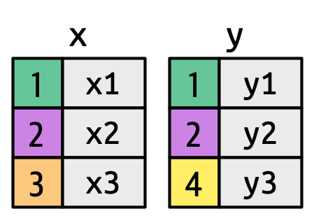
x and y are two data frames with 2 columns and 3 rows, with contents as described in the text. The values of the keys are colored: 1 is green, 2 is purple, 3 is orange, and 4 is yellow. — Figure 19.2: Graphical representation of two simple tables. The colored `key` columns map background color to key value. The grey columns represent the “value” columns that are carried along for the ride.

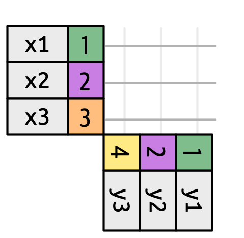
Figure 19.3 展示了我们可视化表示的基础。它显示了 x 和 y 之间所有可能的匹配，即从 x 的每一行和 y 的每一行绘制的线条的交集。输出中的行和列主要由 x 决定，因此 x 表是水平的，并与输出对齐。

x and y are placed at right-angles, with horizonal lines extending from x and vertical lines extending from y. There are 3 rows in x and 3 rows in y, which leads to nine intersections representing nine potential matches. — Figure 19.3: To understand how joins work, it’s useful to think of every possible match. Here we show that with a grid of connecting lines.

为了描述特定类型的连接，我们用点表示匹配。匹配决定了输出中的行，输出是一个包含键、x 值和 y 值的新数据框。例如，Figure 19.4 显示了一个内连接，其中仅当键相等时才保留行。

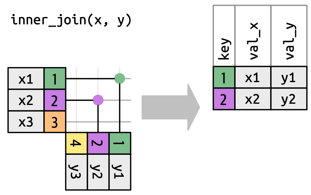
x and y are placed at right-angles with lines forming a grid of potential matches. Keys 1 and 2 appear in both x and y, so we get a match, indicated by a dot. Each dot corresponds to a row in the output, so the resulting joined data frame has two rows. — Figure 19.4: An inner join matches each row in `x` to the row in `y` that has the same value of `key`. Each match becomes a row in the output.

我们可以应用相同的原理来解释外连接，这些连接保留出现在至少一个数据框中的观测。这些连接通过向每个数据框添加一个额外的“虚拟”观测来实现。该观测有一个键，仅当没有其他键匹配时才会匹配，并且值用 NA 填充。外连接有三种类型：

左连接（left join）保留 x 中的所有观测（Figure 19.5）。 x 的每一行都保留在输出中，因为它可以回退到与 y 中的一行 NAs 匹配。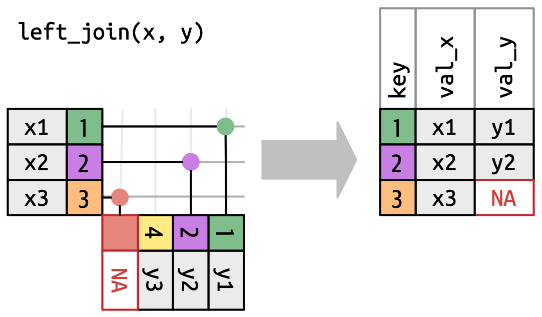

Figure 19.5: A visual representation of the left join where every row in x appears in the output.
右连接（right join）保留 y 中的所有观测（Figure 19.6）。 y 的每一行都保留在输出中，因为它可以回退到与 x 中的一行 NA 匹配。输出仍然尽可能与 x 匹配；来自 y 的任何额外行都会添加到末尾。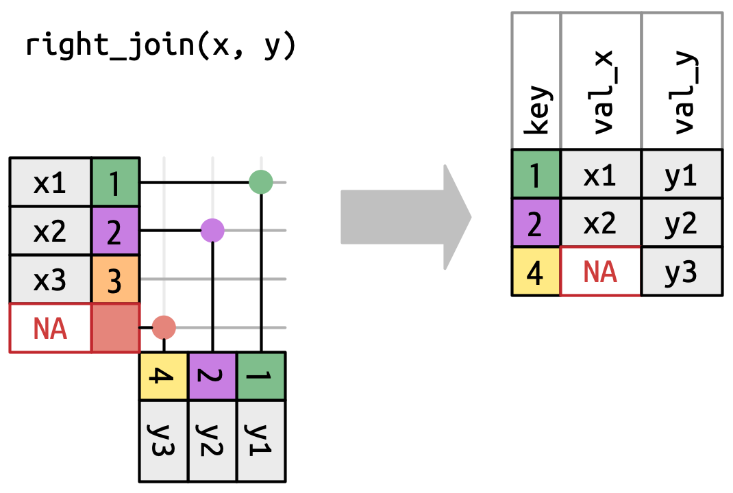

Figure 19.6: A visual representation of the right join where every row of y appears in the output.
全连接（full join）保留出现在 x 或 y 中的所有观测（Figure 19.7）。 x 和 y 的每一行都包含在输出中，因为 x 和 y 都有一个回退的 NA 行。同样，输出从 x 的所有行开始，然后是剩余未匹配的 y 行。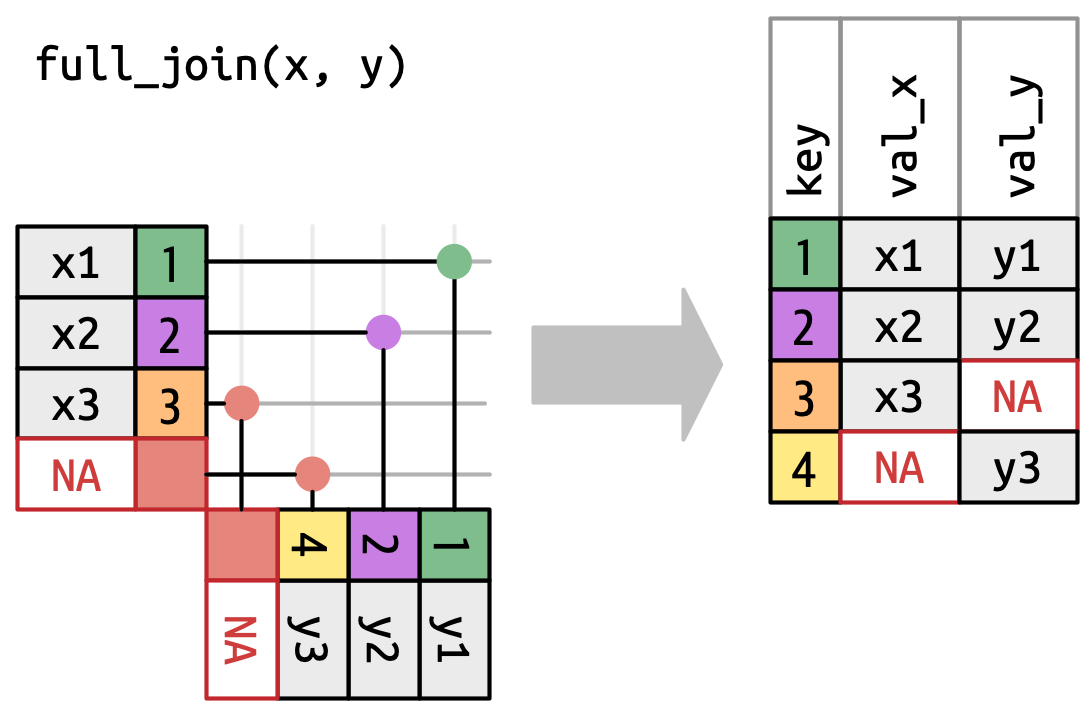

Figure 19.7: A visual representation of the full join where every row in x and y appears in the output.

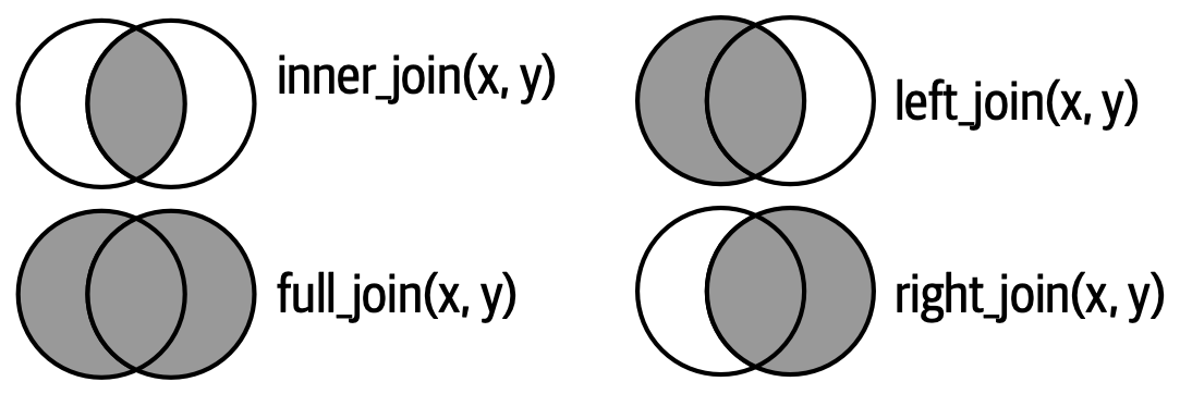
另一种展示不同类型外连接差异的方式是使用维恩图，如 Figure 19.8 所示。然而，这并不是一个很好的表示方式，因为它可能只能唤起你对哪些行被保留的记忆，但无法说明列发生了什么变化。

Venn diagrams for inner, full, left, and right joins. Each join represented with two intersecting circles representing data frames x and y, with x on the right and y on the left. Shading indicates the result of the join. — Figure 19.8: Venn diagrams showing the difference between inner, left, right, and full joins.

这里展示的连接是所谓的等值连接，即当键相等时行匹配。等值连接是最常见的连接类型，因此我们通常会省略“等值”前缀，直接说“内连接”而不是“等值内连接”。我们将在 Section 19.5 中讨论非等值连接。

19.4.1 Row matching

到目前为止，我们探讨了当 x 中的一行匹配 y 中的零行或一行时会发生什么。如果它匹配多于一行会怎样呢？为了理解其中的情况，我们先缩小范围到 inner_join()，然后绘制一张图，如 Figure 19.9 所示。

A join diagram where x has key values 1, 2, and 3, and y has key values 1, 2, 2. The output has three rows because key 1 matches one row, key 2 matches two rows, and key 3 matches zero rows. — Figure 19.9: The three ways a row in `x` can match. `x1` matches one row in `y`, `x2` matches two rows in `y`, `x3` matches zero rows in y. Note that while there are three rows in `x` and three rows in the output, there isn’t a direct correspondence between the rows.

对于 x 中的一行，有三种可能的结果：

如果它没有匹配到任何行，它将被丢弃。
如果它匹配到 y 中的一行，它将被保留。
如果它匹配到 y 中的多行，它会为每个匹配重复一次。

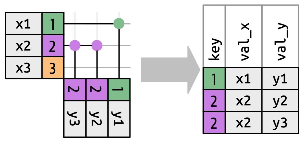
原则上，这意味着输出中的行与 x 中的行之间没有保证的对应关系，但在实践中，这很少引起问题。然而，有一种特别危险的情况可能导致行数的组合爆炸。想象一下连接以下两个表：

df1 <- tibble(key = c(1, 2, 2), val_x = c("x1", "x2", "x3"))
df2 <- tibble(key = c(1, 2, 2), val_y = c("y1", "y2", "y3"))

虽然 df1 中的第一行只匹配 df2 中的一行，但第二行和第三行都匹配两行。这有时被称为 many-to-many 连接，dplyr 会发出警告：

df1 |> 
  inner_join(df2, join_by(key))
#> Warning in inner_join(df1, df2, join_by(key)): Detected an unexpected many-to-many relationship between `x` and `y`.
#> ℹ Row 2 of `x` matches multiple rows in `y`.
#> ℹ Row 2 of `y` matches multiple rows in `x`.
#> ℹ If a many-to-many relationship is expected, set `relationship =
#>   "many-to-many"` to silence this warning.
#> # A tibble: 5 × 3
#>     key val_x val_y
#>   <dbl> <chr> <chr>
#> 1     1 x1    y1   
#> 2     2 x2    y2   
#> 3     2 x2    y3   
#> 4     2 x3    y2   
#> 5     2 x3    y3

如果你是有意这样做的，可以按照警告的建议，设置 relationship = "many-to-many"。

19.4.2 Filtering joins

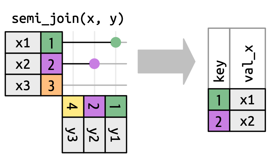
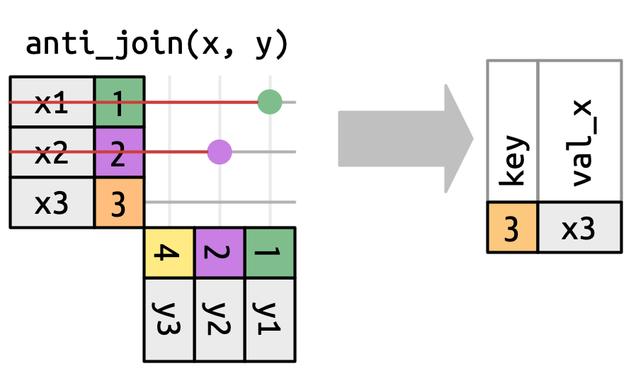
匹配的数量也决定了筛选连接的行为。半连接保留 x 中在 y 中有一个或多个匹配的行，如 Figure 19.10 所示。反连接保留 x 中在 y 中匹配零行的行，如 Figure 19.11 所示。在这两种情况下，重要的是匹配是否存在；匹配多少次并不重要。这意味着筛选连接永远不会像变异连接那样重复行。

A join diagram with old friends x and y. In a semi join, only the presence of a match matters so the output contains the same columns as x. — Figure 19.10: In a semi-join it only matters that there is a match; otherwise values in `y` don’t affect the output.

An anti-join is the inverse of a semi-join so matches are drawn with red lines indicating that they will be dropped from the output. — Figure 19.11: An anti-join is the inverse of a semi-join, dropping rows from `x` that have a match in `y`.

19.5 Non-equi joins

到目前为止，你只见过等值连接，即当 x 键等于 y 键时行匹配的连接。现在我们将放宽这个限制，讨论其他确定一对行是否匹配的方法。

但在我们这样做之前，我们需要重新审视之前的一个简化。在等值连接中，x 键和 y 键总是相等的，因此我们只需要在输出中显示一个键。我们可以要求 dplyr 用 keep = TRUE 保留两个键，导致下面的代码和在 Figure 19.12 中重新绘制的 inner_join()。

x |> left_join(y, by = "key", keep = TRUE)
#> # A tibble: 3 × 4
#>   key.x val_x key.y val_y
#>   <dbl> <chr> <dbl> <chr>
#> 1     1 x1        1 y1   
#> 2     2 x2        2 y2   
#> 3     3 x3       NA <NA>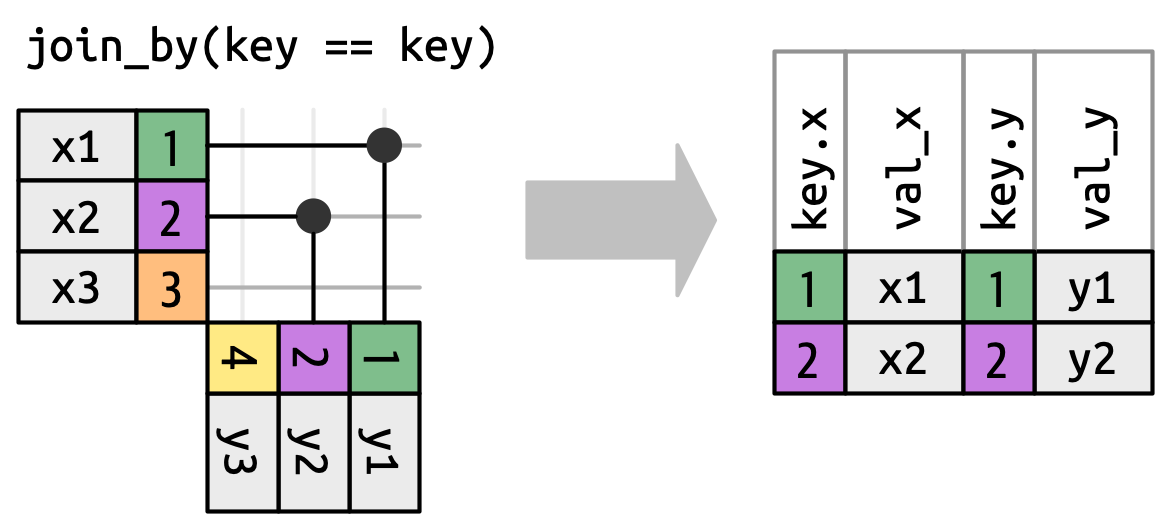

A join diagram showing an inner join betwen x and y. The result now includes four columns: key.x, val_x, key.y, and val_y. The values of key.x and key.y are identical, which is why we usually only show one. — Figure 19.12: An inner join showing both `x` and `y` keys in the output.

当我们离开等值连接时，我们将总是显示两个键，因为键值通常会不同。例如，我们不再仅仅在 x$key 和 y$key 相等时匹配，而是在 x$key 大于或等于 y$key 时匹配，导致 Figure 19.13。 dplyr 的连接函数理解等值连接和非等值连接之间的区别，因此当你执行非等值连接时，它总是显示两个键。

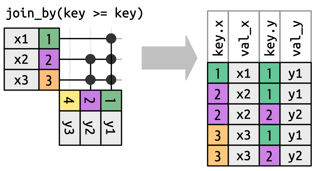
A join diagram illustrating join_by(key >= key). The first row of x matches one row of y and the second and thirds rows each match two rows. This means the output has five rows containing each of the following (key.x, key.y) pairs: (1, 1), (2, 1), (2, 2), (3, 1), (3, 2). — Figure 19.13: A non-equi join where the `x` key must be greater than or equal to the `y` key. Many rows generate multiple matches.

“非等值连接”并不是一个特别有用的术语，因为它只告诉你连接不是什么，而不是它是什么。d plyr 通过识别四种特别有用的非等值连接类型来提供帮助：

交叉连接（Cross joins）匹配每一对行。
不等式连接（Inequality joins）使用 <, <=, > 和 >= 而不是 ==。
滚动连接（Rolling joins）类似于不等式连接，但只找到最接近的匹配。
重叠连接（Overlap joins）是一种特殊类型的不等式连接，设计用于处理范围。

以下各节将更详细地描述这些类型。

19.5.1 Cross joins

交叉连接会匹配所有内容，如 Figure 19.14 所示，生成行的笛卡尔积。这意味着输出将有 nrow(x) * nrow(y) 行。

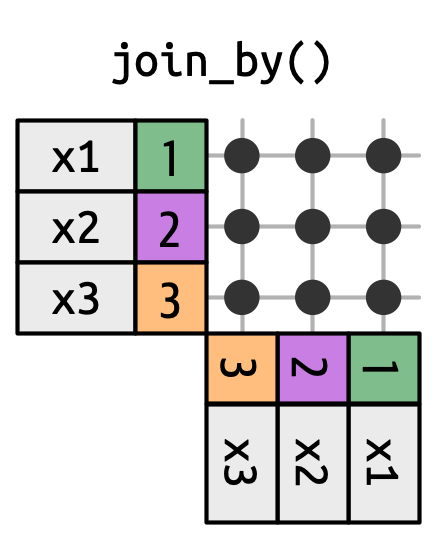
A join diagram showing a dot for every combination of x and y. — Figure 19.14: A cross join matches each row in `x` with every row in `y`.

交叉连接在生成排列组合时很有用。例如，下面的代码生成了所有可能的名字对。由于我们将 df 与自身连接，这有时被称为自连接。交叉连接使用不同的连接函数，因为当匹配每一行时，内/左/右/全连接之间没有区别。

df <- tibble(name = c("John", "Simon", "Tracy", "Max"))
df |> cross_join(df)
#> # A tibble: 16 × 2
#>   name.x name.y
#>   <chr>  <chr> 
#> 1 John   John  
#> 2 John   Simon 
#> 3 John   Tracy 
#> 4 John   Max   
#> 5 Simon  John  
#> 6 Simon  Simon 
#> # ℹ 10 more rows

19.5.2 Inequality joins

不等式连接使用 <, <=, >= 或 > 来限制可能的匹配集，如 Figure 19.13 和 Figure 19.15 所示。

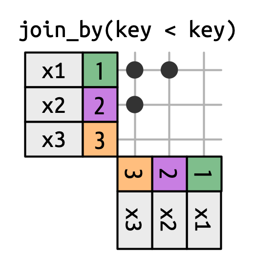
A diagram depicting an inequality join where a data frame x is joined by a data frame y where the key of x is less than the key of y, resulting in a triangular shape in the top-left corner. — Figure 19.15: An inequality join where `x` is joined to `y` on rows where the key of `x` is less than the key of `y`. This makes a triangular shape in the top-left corner.

不等式连接极其通用，通用到很难提出有意义的特定用例。一个有用的技巧是使用它们来限制交叉连接，从而生成所有组合而非所有排列：

df <- tibble(id = 1:4, name = c("John", "Simon", "Tracy", "Max"))

df |> left_join(df, join_by(id < id))
#> # A tibble: 7 × 4
#>    id.x name.x  id.y name.y
#>   <int> <chr>  <int> <chr> 
#> 1     1 John       2 Simon 
#> 2     1 John       3 Tracy 
#> 3     1 John       4 Max   
#> 4     2 Simon      3 Tracy 
#> 5     2 Simon      4 Max   
#> 6     3 Tracy      4 Max   
#> # ℹ 1 more row

19.5.3 Rolling joins

滚动连接是一种特殊类型的不等式连接，它不是获取每个满足不等式的行，而是只获取最接近的行，如 Figure 19.16 所示。你可以通过添加 closest() 将任何不等式连接转换为滚动连接。例如，join_by(closest(x <= y)) 匹配大于或等于 x 的最小 y，而 join_by(closest(x > y)) 匹配小于 x 的最大 y。

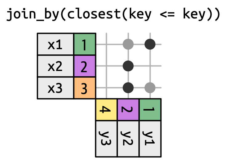
A rolling join is a subset of an inequality join so some matches are grayed out indicating that they're not used because they're not the "closest". — Figure 19.16: A rolling join is similar to a greater-than-or-equal inequality join but only matches the first value.

当你有两个日期不完全对齐的表，并且想找到表 1 中最接近表 2 中某个日期之前（或之后）的日期时，滚动连接特别有用。

例如，假设你负责公司的派对策划委员会。你的公司相当节俭，因此不举办单独的派对，而是每季度只举办一次。确定派对举行时间的规则有些复杂：派对总是在周一举行，一月的第一周因很多人休假而跳过，2022年第三季度的第一个周一是7月4日，因此必须推迟一周。这导致了以下派对日期：

parties <- tibble(
  q = 1:4,
  party = ymd(c("2022-01-10", "2022-04-04", "2022-07-11", "2022-10-03"))
)

现在假设你有一个员工生日表：

employees <- tibble(
  name = sample(babynames::babynames$name, 100),
  birthday = ymd("2022-01-01") + (sample(365, 100, replace = TRUE) - 1)
)
employees
#> # A tibble: 100 × 2
#>   name    birthday  
#>   <chr>   <date>    
#> 1 Case    2022-09-13
#> 2 Shonnie 2022-03-30
#> 3 Burnard 2022-01-10
#> 4 Omer    2022-11-25
#> 5 Hillel  2022-07-30
#> 6 Curlie  2022-12-11
#> # ℹ 94 more rows

我们想为每位员工找到生日之后（或当天）的第一个派对日期。我们可以用滚动连接来表达这一点：

employees |> 
  left_join(parties, join_by(closest(birthday >= party)))
#> # A tibble: 100 × 4
#>   name    birthday       q party     
#>   <chr>   <date>     <int> <date>    
#> 1 Case    2022-09-13     3 2022-07-11
#> 2 Shonnie 2022-03-30     1 2022-01-10
#> 3 Burnard 2022-01-10     1 2022-01-10
#> 4 Omer    2022-11-25     4 2022-10-03
#> 5 Hillel  2022-07-30     3 2022-07-11
#> 6 Curlie  2022-12-11     4 2022-10-03
#> # ℹ 94 more rows

然而，这种方法有一个问题：生日在1月10日之前的员工没有分配到派对：

employees |> 
  anti_join(parties, join_by(closest(birthday >= party)))
#> # A tibble: 0 × 2
#> # ℹ 2 variables: name <chr>, birthday <date>

为了解决这个问题，我们需要用另一种方式处理，即使用重叠连接。

19.5.4 Overlap joins

重叠连接提供了三个辅助函数，它们利用不等式连接来更便捷地处理区间：

between(x, y_lower, y_upper) 是 x >= y_lower, x <= y_upper 的简写.
within(x_lower, x_upper, y_lower, y_upper) 是 x_lower >= y_lower, x_upper <= y_upper 的简写.
overlaps(x_lower, x_upper, y_lower, y_upper) 是 x_lower <= y_upper, x_upper >= y_lower 的简写.

我们继续生日示例，看看如何使用它们。我们之前使用的策略有一个问题：1月1日至9日的生日没有对应的派对。因此，最好明确每个派对涵盖的日期范围，并为这些早期生日设置特殊处理：

parties <- tibble(
  q = 1:4,
  party = ymd(c("2022-01-10", "2022-04-04", "2022-07-11", "2022-10-03")),
  start = ymd(c("2022-01-01", "2022-04-04", "2022-07-11", "2022-10-03")),
  end = ymd(c("2022-04-03", "2022-07-11", "2022-10-02", "2022-12-31"))
)
parties
#> # A tibble: 4 × 4
#>       q party      start      end       
#>   <int> <date>     <date>     <date>    
#> 1     1 2022-01-10 2022-01-01 2022-04-03
#> 2     2 2022-04-04 2022-04-04 2022-07-11
#> 3     3 2022-07-11 2022-07-11 2022-10-02
#> 4     4 2022-10-03 2022-10-03 2022-12-31

Hadley 在数据录入方面糟糕透顶，他还想检查派对时段是否重叠。一种方法是使用自连接来检查任何起止区间是否与其他区间重叠：

parties |> 
  inner_join(parties, join_by(overlaps(start, end, start, end), q < q)) |> 
  select(start.x, end.x, start.y, end.y)
#> # A tibble: 1 × 4
#>   start.x    end.x      start.y    end.y     
#>   <date>     <date>     <date>     <date>    
#> 1 2022-04-04 2022-07-11 2022-07-11 2022-10-02

哎呀，确实存在重叠，所以让我们修复这个问题并继续：

parties <- tibble(
  q = 1:4,
  party = ymd(c("2022-01-10", "2022-04-04", "2022-07-11", "2022-10-03")),
  start = ymd(c("2022-01-01", "2022-04-04", "2022-07-11", "2022-10-03")),
  end = ymd(c("2022-04-03", "2022-07-10", "2022-10-02", "2022-12-31"))
)

现在我们可以为每位员工匹配他们的派对了。这是一个使用 unmatched = "error" 的好时机，因为我们希望快速发现是否有员工未被分配派对。

employees |> 
  inner_join(parties, join_by(between(birthday, start, end)), unmatched = "error")
#> # A tibble: 100 × 6
#>   name    birthday       q party      start      end       
#>   <chr>   <date>     <int> <date>     <date>     <date>    
#> 1 Case    2022-09-13     3 2022-07-11 2022-07-11 2022-10-02
#> 2 Shonnie 2022-03-30     1 2022-01-10 2022-01-01 2022-04-03
#> 3 Burnard 2022-01-10     1 2022-01-10 2022-01-01 2022-04-03
#> 4 Omer    2022-11-25     4 2022-10-03 2022-10-03 2022-12-31
#> 5 Hillel  2022-07-30     3 2022-07-11 2022-07-11 2022-10-02
#> 6 Curlie  2022-12-11     4 2022-10-03 2022-10-03 2022-12-31
#> # ℹ 94 more rows

19.5.5 Exercises

你能解释在这个等值连接中键发生了什么情况吗？为什么它们会不同？

x |> full_join(y, by = "key")
#> # A tibble: 4 × 3
#>     key val_x val_y
#>   <dbl> <chr> <chr>
#> 1     1 x1    y1   
#> 2     2 x2    y2   
#> 3     3 x3    <NA> 
#> 4     4 <NA>  y3

x |> full_join(y, by = "key", keep = TRUE)
#> # A tibble: 4 × 4
#>   key.x val_x key.y val_y
#>   <dbl> <chr> <dbl> <chr>
#> 1     1 x1        1 y1   
#> 2     2 x2        2 y2   
#> 3     3 x3       NA <NA> 
#> 4    NA <NA>      4 y3

在查找是否有派对时间段与其他派对时间段重叠时，我们在 join_by() 中使用了 q < q？为什么？如果移除这个不等式会发生什么？

19.6 Summary

在本章中，你学习了如何使用变异连接和筛选连接来合并两个数据框的数据。过程中你学会了如何识别键，以及主键和外键的区别。你还理解了连接的工作原理，以及如何推断输出将有多少行。最后，你初步见识了非等值连接的强大功能，并看到了一些有趣的用例。

本章结束了本书的“转换”部分，该部分的重点在于可用于处理单个列和 tibble 的工具。你学习了用于处理逻辑向量、数字和完整表格的 dplyr 及基础函数，用于处理字符串的 stringr 函数，用于处理日期时间的 lubridate 函数，以及用于处理因子的 forcats 函数。

在本书的下一部分，你将学习更多关于将各类数据以整洁形式导入 R 的知识。

记住，在 RStudio 中，你也可以使用 View() 来避免这个问题。↩︎
这并不是百分百正确，但如果不是，你就会得到警告。↩︎