10  Exploratory data analysis

10.1 Introduction

本章将向您展示如何使用可视化和转换以系统的方式探索数据，统计学家将这项任务称为探索性数据分析（exploratory data analysis），简称 EDA。 EDA 是一个迭代循环。 你：

1. 提出有关您的数据的问题。

2. 通过可视化、转换和建模数据来搜索答案。

3. 使用您学到的知识来完善您的问题和/或产生新问题。

EDA 不是一个具有严格规则的正式流程。 最重要的是，EDA 是一种心态。 在 EDA 的初始阶段，您应该随意调查您想到的每个想法。 其中一些想法会成功，而另一些则会是死胡同。 随着探索的继续，您将获得一些特别富有成效的见解，最终将其写下来并与其他人交流。

EDA 是任何数据分析的重要组成部分，即使主要的研究问题已经摆在您面前，因为您始终需要调查数据的质量。 数据清理只是 EDA 的一种应用：您询问数据是否符合您的期望。 要进行数据清理，您需要部署 EDA 的所有工具：可视化、转换和建模。

10.1.1 Prerequisites

在本章中，我们将结合您所学到的有关 dplyr 和 ggplot2 的知识来交互式地提出问题，用数据回答它们，然后提出新问题。

library(tidyverse)

10.2 Questions

“There are no routine statistical questions, only questionable statistical routines.” — Sir David Cox

“Far better an approximate answer to the right question, which is often vague, than an exact answer to the wrong question, which can always be made precise.” — John Tukey

您在 EDA 期间的目标是加深对数据的理解。 最简单的方法是使用问题作为指导调查的工具。 当您提出问题时，该问题会将您的注意力集中在数据集的特定部分上，并帮助您决定要进行哪些图形、模型或转换。

EDA 从根本上来说是一个创造性的过程。 与大多数创意过程一样，提出高质量问题的关键是产生大量问题。 在分析开始时很难提出有启发性的问题，因为您不知道可以从数据集中收集哪些见解。 另一方面，您提出的每个新问题都会让您接触到数据的新方面，并增加您做出发现的机会。 如果您根据发现的内容提出一个新问题来跟进每个问题，则可以快速深入了解数据中最有趣的部分，并提出一组发人深省的问题。

对于应该提出哪些问题来指导您的研究，没有任何规定。 然而，有两种类型的问题对于在数据中进行发现总是有用的。 您可以将这些问题大致表述为：

1. 我的变量中发生什么类型的变化？

2. 我的变量之间发生什么类型的共同变化？

本章的其余部分将讨论这两个问题。 我们将解释什么是变化（variation）和共同变化（covariation），并向您展示回答每个问题的几种方法。

10.3 Variation

Variation 是变量值在不同测量中发生变化的趋势。 在现实生活中你可以很容易地看到 variation；如果您两次测量任何连续变量，您将得到两个不同的结果。 即使您测量的是恒定量情况也是如此，例如光速。 您的每次测量都会包含少量误差，该误差因测量而异。 如果您在不同的对象（例如，不同人的眼睛颜色）或在不同的时间（例如，不同时刻的电子能级）进行测量，变量也会有所不同。 每个变量都有自己的变化模式，这可以揭示有关同一观察的测量之间以及不同观察之间的变化的有趣信息。 理解该模式的最佳方法是可视化变量值的分布，您已在 Chapter 1 中了解了这一点。

我们将通过可视化 diamonds 数据集中 ~54,000 颗钻石的重量（carat）分布来开始我们的探索。 由于 carat 是一个数值变量，我们可以使用直方图（histogram）：

ggplot(diamonds, aes(x = carat)) +
  geom_histogram(binwidth = 0.5)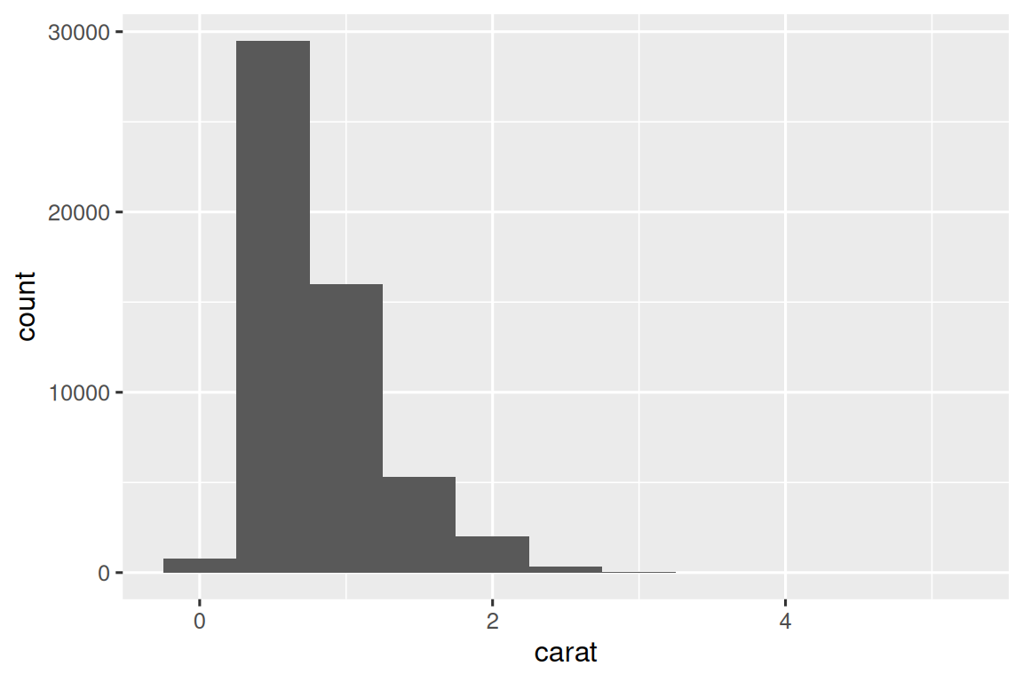

现在您可以可视化 variation，您应该在图中寻找什么？ 您应该提出什么类型的后续问题？ 我们在下面列出了您将在图表中找到的最有用的信息类型，以及针对每种信息类型的一些后续问题。 提出好的后续问题的关键是依靠你的好奇心（你想了解更多什么？）以及你的怀疑精神（这怎么可能误导？）。

10.3.1 Typical values

在条形图和直方图中，高条形显示变量的常见值，较短的条形显示不太常见的值。 没有条形的位置显示数据中未看到的值。 要将这些信息转化为有用的问题，请寻找任何意想不到的东西：

• 哪些值最常见？ 为什么？

• 哪些值是稀有的？ 为什么？ 这符合您的期望吗？

• 你能看到任何不寻常的模式吗？ 什么可以解释它们？

让我们看一下较小钻石的 carat 分布。

smaller <- diamonds |> 
  filter(carat < 3)

ggplot(smaller, aes(x = carat)) +
  geom_histogram(binwidth = 0.01)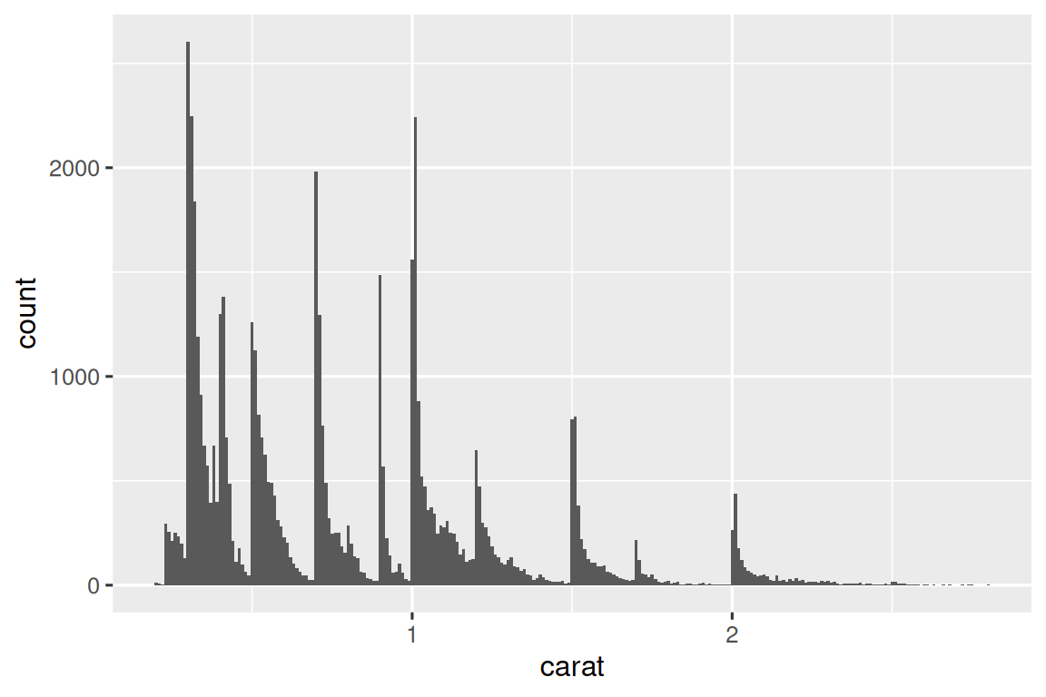

该直方图提出了几个有趣的问题：

• 为什么整克拉和常见分数克拉的钻石更多？

• 为什么每个峰稍右侧的菱形数量多于每个峰左侧的菱形数量？

可视化还可以揭示 clusters，这表明数据中存在 subgroups。 要了解 subgroups，请询问：

• 每个 subgroup 内的观察结果有何相似之处？

• 不同 clusters 中的观察结果有何不同？

• 您如何解释或描述这些 clusters？

• 为什么 clusters 的出现可能会产生误导？

其中一些问题可以通过数据来回答，而另一些则需要有关数据的领域专业知识。 其中许多会提示您探索变量之间的关系，例如，看看一个变量的值是否可以解释另一个变量的行为。 我们很快就会谈到这一点。

10.3.2 Unusual values

异常值（Outliers）是指不寻常的观察结果；数据点似乎不符合模式。 有时异常值是数据输入错误，有时它们只是在此数据收集中碰巧观察到的极端值，有时它们表明了重要的新发现。 当您有大量数据时，有时很难在直方图中看到异常值。 例如，从 diamonds 数据集中获取 y 变量的分布。 异常值的唯一证据是 x-axis 上异常宽的限制。

ggplot(diamonds, aes(x = y)) + 
  geom_histogram(binwidth = 0.5)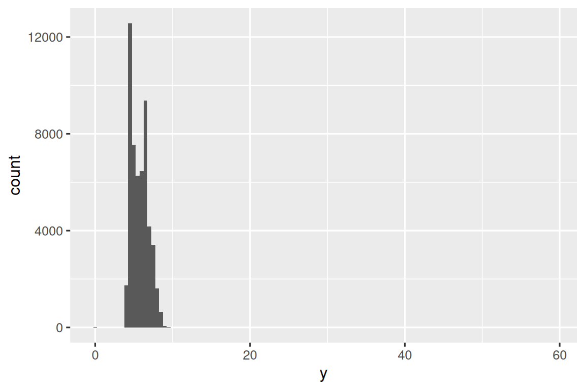

常见的 bin 中有太多的观察结果，而稀有的 bin 则非常短，因此很难看到它们（尽管如果你专心地盯着 0，也许你会发现一些东西）。 为了更容易看到不寻常的值，我们需要使用 coord_cartesian() 缩放到 y-axis 的小值：

ggplot(diamonds, aes(x = y)) + 
  geom_histogram(binwidth = 0.5) +
  coord_cartesian(ylim = c(0, 50))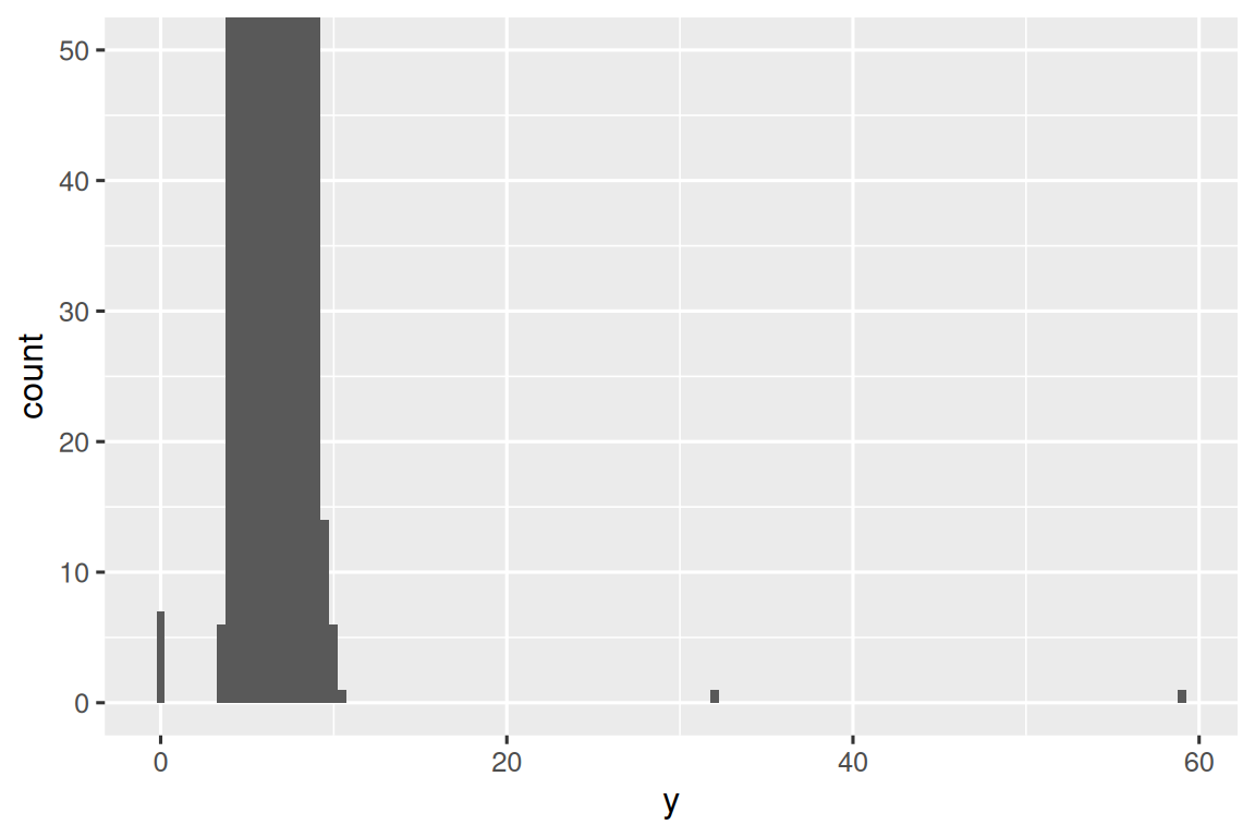

coord_cartesian() 还有一个 xlim() 参数，用于当您需要放大 x 轴时。 ggplot2 还具有 xlim() 和 ylim() 函数，它们的工作方式略有不同：它们丢弃超出限制的数据。

这让我们可以看到存在三个不寻常的值：0, ~30, and ~60。 我们用 dplyr 将它们取出：

unusual <- diamonds |> 
  filter(y < 3 | y > 20) |> 
  select(price, x, y, z) |>
  arrange(y)
unusual
#> # A tibble: 9 × 4
#>   price     x     y     z
#>   <int> <dbl> <dbl> <dbl>
#> 1  5139  0      0    0   
#> 2  6381  0      0    0   
#> 3 12800  0      0    0   
#> 4 15686  0      0    0   
#> 5 18034  0      0    0   
#> 6  2130  0      0    0   
#> 7  2130  0      0    0   
#> 8  2075  5.15  31.8  5.12
#> 9 12210  8.09  58.9  8.06

y 变量测量这些钻石的三个尺寸之一，以 mm 为单位。 我们知道钻石的宽度不可能是 0mm，所以这些值一定是不正确的。 通过 EDA，我们发现了编码为 0 的缺失数据，这是我们通过简单搜索 NAs 永远无法找到的。 展望未来，我们可能会选择将这些值重新编码为 NAs，以防止误导计算。 我们可能还会怀疑 32mm 和 59mm 的测量结果令人难以置信：这些钻石超过一英寸长，但价格却不用花费数十万美元！

在有或没有异常值的情况下重复分析是一个很好的做法。 如果它们对结果的影响很小，并且您无法弄清楚它们为什么在那里，那么忽略它们并继续前进是合理的。 然而，如果它们对你的结果有重大影响，你不应该无缘无故地放弃它们。 您需要找出导致它们的原因（例如数据输入错误），并披露您在文章中删除了它们。

10.3.3 Exercises

1. 探索钻石中每个 x、y 和 z 变量的分布。 你学到了什么？ 想象一下钻石，以及如何确定长度、宽度和深度的尺寸。

2. 探索 price 分布。 您是否发现任何不寻常或令人惊讶的事情？ （提示：仔细考虑 binwidth 并确保尝试广泛的值。）

3. 0.99 克拉有多少颗钻石？ 1 克拉是多少？ 您认为造成这种差异的原因是什么？

4. 放大直方图时，比较和对比 coord_cartesian() 与 xlim() 或 ylim()。 如果未设置 binwidth 会发生什么？ 如果您尝试缩放，只显示半条，会发生什么情况？

10.4 Unusual values

如果您在数据集中遇到了异常值，并且只想继续进行其余的分析，您有两种选择。

1. 删除具有奇怪值的整行：

   diamonds2 <- diamonds |> 
     filter(between(y, 3, 20))

   我们不推荐此选项，因为一个无效值并不意味着该观察的所有其他值也无效。 此外，如果您的数据质量较低，当您将此方法应用于每个变量时，您可能会发现您没有任何数据了！

2. 相反，我们建议用缺失值替换异常值。 最简单的方法是使用 mutate() 用修改后的副本替换变量。 您可以使用 if_else() 函数将异常值替换为 NA：

   diamonds2 <- diamonds |> 
     mutate(y = if_else(y < 3 | y > 20, NA, y))

应该在哪里绘制缺失值并不明显，因此 ggplot2 不会将它们包含在图中，但它确实警告它们已被删除：

ggplot(diamonds2, aes(x = x, y = y)) + 
  geom_point()
#> Warning: Removed 9 rows containing missing values or values outside the scale range
#> (`geom_point()`).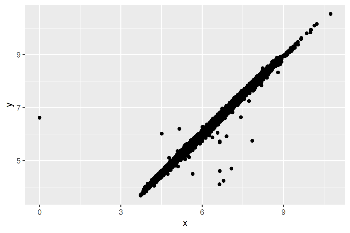

要抑制该警告，请设置 na.rm = TRUE：

ggplot(diamonds2, aes(x = x, y = y)) + 
  geom_point(na.rm = TRUE)

其他时候，您想要了解是什么使具有缺失值的观测值与具有记录值的观测值不同。 例如，在 nycflights13::flights¹ 中，dep_time 变量中缺失值表示航班已取消。 因此，您可能需要比较已取消和未取消的预定出发时间。 您可以通过创建一个新变量，使用 is.na() 检查 dep_time 是否丢失来做到这一点。

nycflights13::flights |> 
  mutate(
    cancelled = is.na(dep_time),
    sched_hour = sched_dep_time %/% 100,
    sched_min = sched_dep_time %% 100,
    sched_dep_time = sched_hour + (sched_min / 60)
  ) |> 
  ggplot(aes(x = sched_dep_time)) + 
  geom_freqpoly(aes(color = cancelled), binwidth = 1/4)

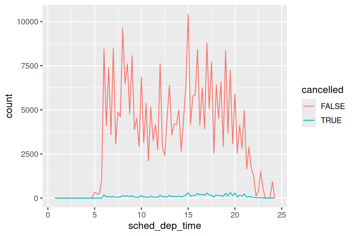
然而，这个图并不好，因为未取消的航班比取消的航班多得多。 在下一节中，我们将探讨一些改进这种比较的技术。

10.4.1 Exercises

1. 直方图中缺失值会怎样？ 条形图中缺失值会发生什么情况？ 为什么直方图和条形图中缺失值的处理方式存在差异？

2. na.rm = TRUE 在 mean() 和 sum() 中做了什么？

3. 重新创建 scheduled_dep_time 的频率图，根据航班是否取消进行着色。 并通过 cancelled 变量进行分面（facet）。 在分面函数中尝试不同的 scales 变量值，以减轻未取消航班多于已取消航班的影响。

10.5 Covariation

若变异（variation）描述的是单个变量内部的变化特征，那么协方差（covariation）则刻画的是多个变量之间的协同变化规律。 协方差（covariation）是两个或更多变量的取值呈现关联性波动的趋势。 要识别协方差（covariation），最有效的方式是将变量间的关联进行可视化呈现。

10.5.1 A categorical and a numerical variable

例如，我们可通过 geom_freqpoly() 函数来探究钻石价格与其品质（以 cut 衡量）的变化关系：

ggplot(diamonds, aes(x = price)) + 
  geom_freqpoly(aes(color = cut), binwidth = 500, linewidth = 0.75)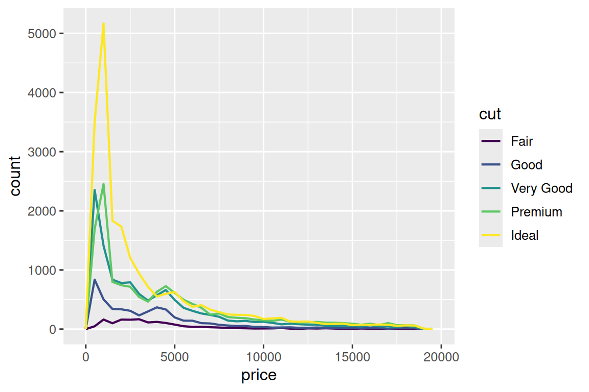

注意由于 cut 在数据中被定义为有序因子变量，ggplot2 自动采用了有序颜色标度，具体原理将在 Section 16.6 详述。

不过 geom_freqpoly() 的默认输出在此场景下效果欠佳由于高度，由计数总量决定，而不同 cuts 等级的样本量差异悬殊，导致分布曲线的形态差异难以辨识。

为提升可比性，我们需要调整 y 轴显示方式。不 是显示绝对计数（count），我们将显示密度值（density）。密 度标准化了计数分布，使得每个频率多边形下的面积为 1。

ggplot(diamonds, aes(x = price, y = after_stat(density))) + 
  geom_freqpoly(aes(color = cut), binwidth = 500, linewidth = 0.75)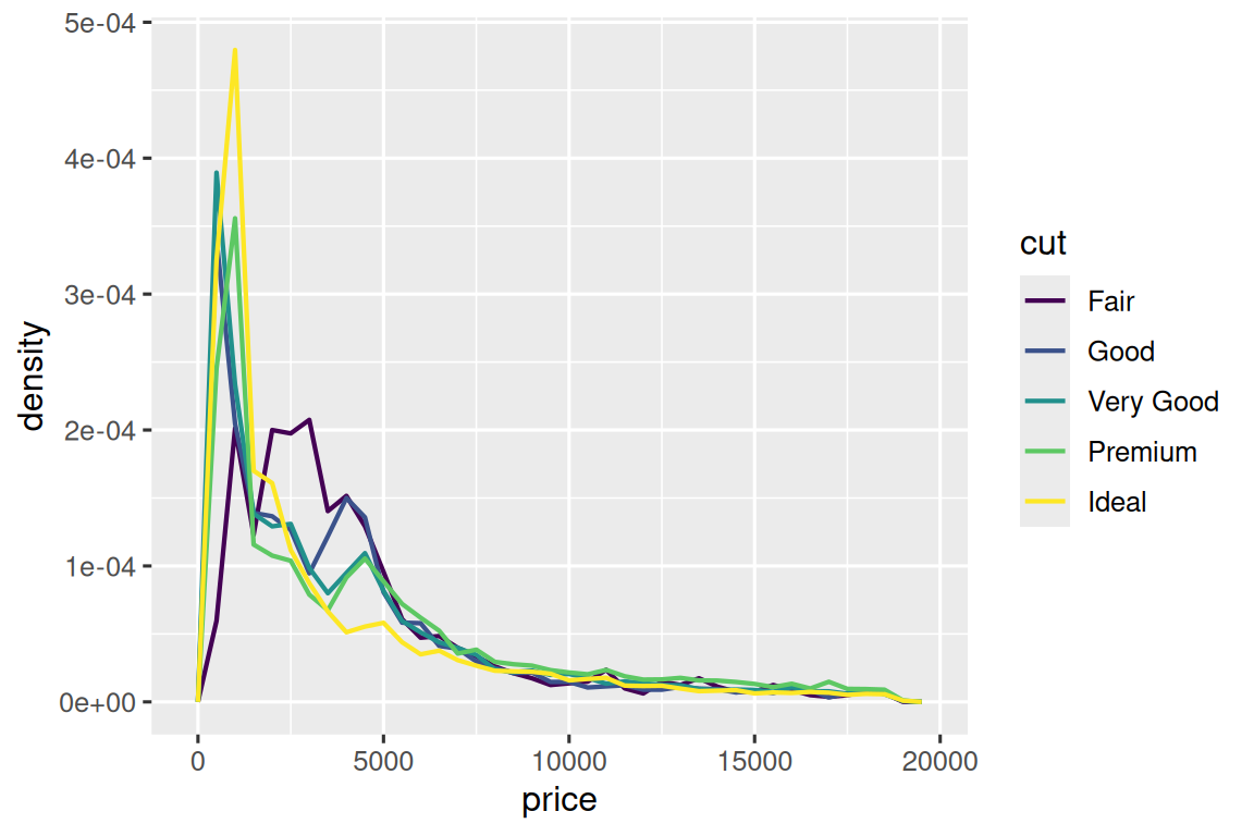

需要特别说明的是，虽然我们将密度（density）映射到 y 轴，但由于原始数据 diamonds 中并不存在 density，我们需要先计算它。 我们使用 after_stat() 函数进行计算。

这个可视化结果揭示了一个反常识现象 - 似乎一般级钻石（质量最低）的平均价格最高！ 但是这可能与频率多边形图的解读难度有关 - 图中重叠的分布曲线确实容易造成视觉混淆。

一种视觉上更简单的图用于探索这种关系是使用并排箱线图。

ggplot(diamonds, aes(x = cut, y = price)) +
  geom_boxplot()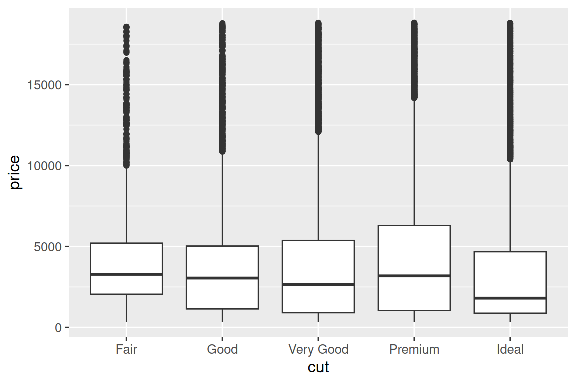

我们看到有分布的信息较少，但是箱线图更紧凑，因此我们可以更轻松地比较它们（且能在一个图中展示更多数据）。 结果再次验证了那个反直觉的发现，即质量较高的钻石通常更便宜！ 在练习中，您将会挑战弄清楚原因。

cut 作为有序因子变量，其等级从一般（fair）、良好（good）、很好（very good）到极好（ideal）具有明确递进关系。 但许多分类变量并不具备这种内在顺序，因此您可能需要重新排序它们以显示更多信息。 一种方法是使用 fct_reorder()。 您将在 Section 16.4 中了解有关该功能的更多信息，但是我们想在这里为您提供快速预览，因为它非常有用。 例如，在 mpg 数据集中使用 class 变量。 您可能有兴趣知道高速公路里程（hwy）在各个车型类别（class）中的变化：

ggplot(mpg, aes(x = class, y = hwy)) +
  geom_boxplot()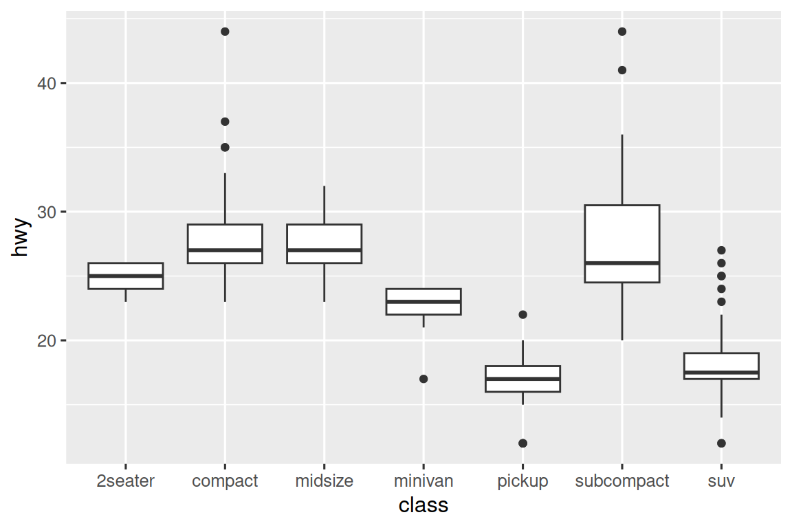

To make the trend easier to see, we can reorder class based on the median value of hwy: 为了使趋势更容易看到，我们可以根据 hwy 的中值重新排序 class：

ggplot(mpg, aes(x = fct_reorder(class, hwy, median), y = hwy)) +
  geom_boxplot()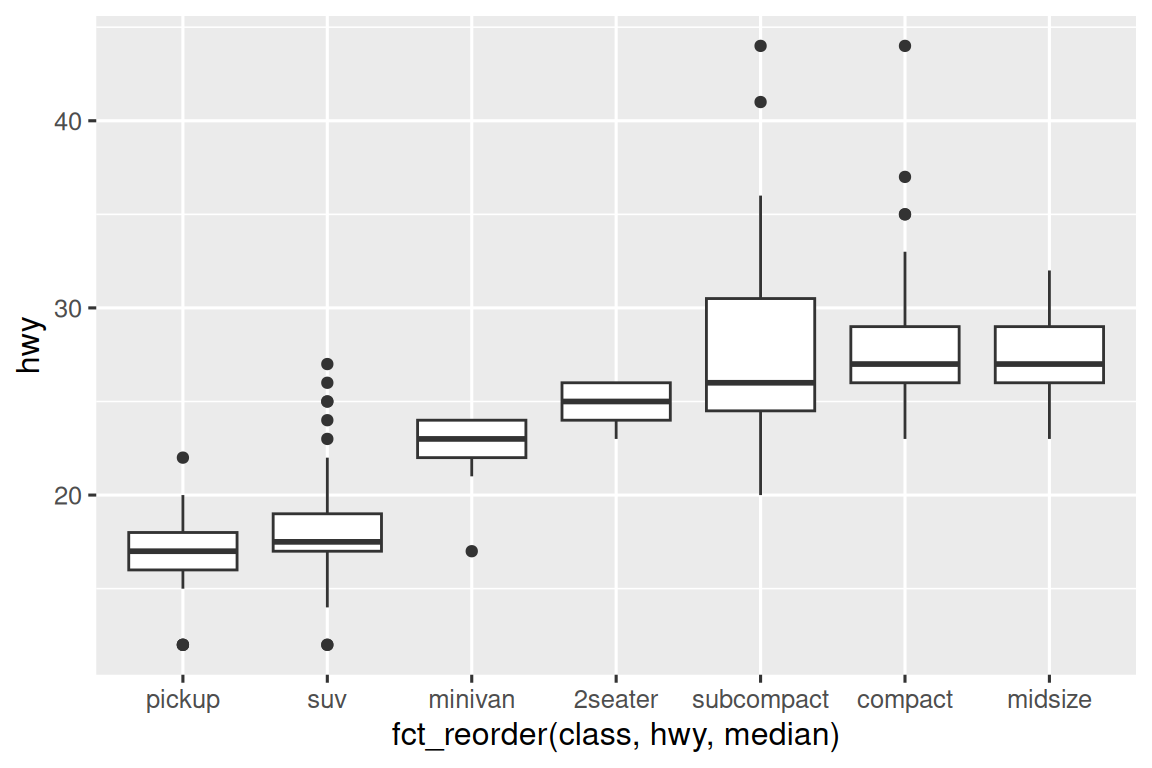

如果您有长变量名，geom_boxplot() 会更好地工作如果你将其翻转 90°。 您可以通过交换 X 和 Y 美学映射来做到这一点。

ggplot(mpg, aes(x = hwy, y = fct_reorder(class, hwy, median))) +
  geom_boxplot()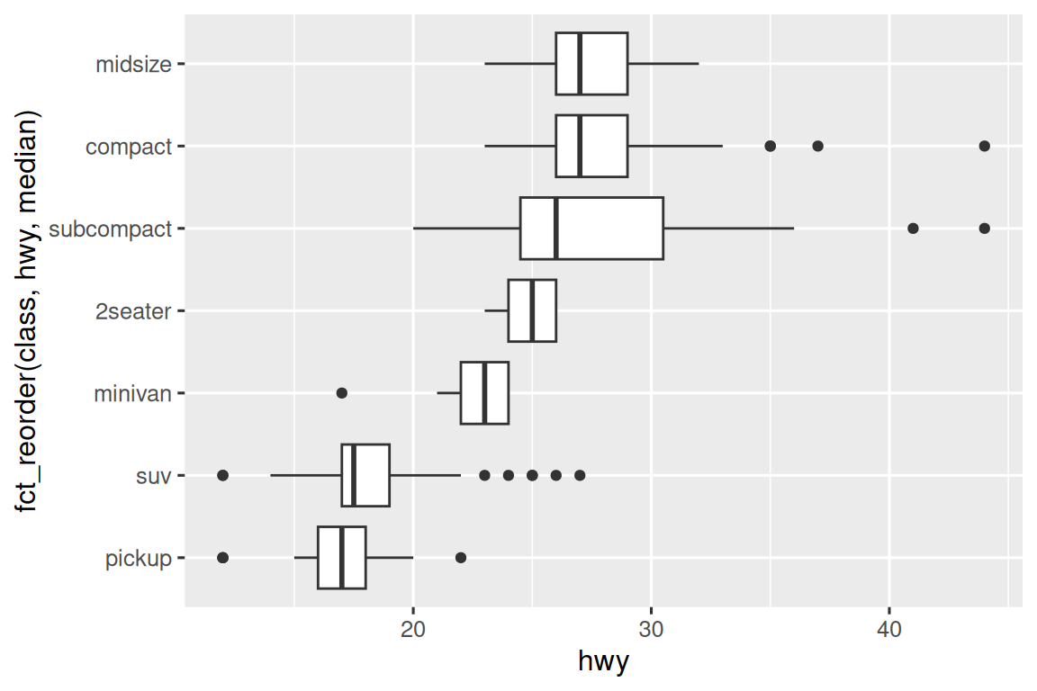

10.5.1.1 Exercises

1. 利用您学到的知识来改善”已取消航班与正常航班起飞时间”的可视化呈现。

2. 根据探索性数据分析（EDA），diamonds数据集中哪个变量对价格预测最具重要性？ 该变量与cut存在何种相关性？ 这两种关系的共同作用如何导致低品质钻石价格更高？

3. 无需调换x/y变量，通过在垂直箱线图中添加coord_flip()图层即可生成水平箱线图。 与直接交换变量的方式相比有何优劣？

4. 箱线图的局限性在于其设计初衷是针对小规模数据集，当处理大数据时会显示过多”离群值（outlying values）“。 改进方案之一是采用字母值图（letter value plot）。 安装lvplot包后，尝试用geom_lv()展示price与cut的关系分布。 你从中学到了什么？ 应如何解读这类图表？

5. 使用geom_violin()从diamonds数据集中创建一个可视化钻石 prices vs. 一个分类变量，然后一个 faceted geom_histogram()，然后一个 colored geom_freqpoly()，然后一个colored geom_density()。 比较和对比四个图。 根据分类变量的级别可视化数值变量的分布的每种方法的利弊是什么？

6. 如果您有一个小数据集，则有时使用geom_jitter()避免过度分布以更轻松地查看连续变量和分类变量之间的关系是有用的。 ggbeeswarm 软件包提供了许多类似于 geom_jitter() 的方法。 列出它们，并简要描述它们每个的作用。

10.5.2 Two categorical variables

为了可视化分类变量之间的协方差，您需要计算这些分类变量级别的每种组合的观测值。 一种方法是依靠内置的 geom_count()：

ggplot(diamonds, aes(x = cut, y = color)) +
  geom_count()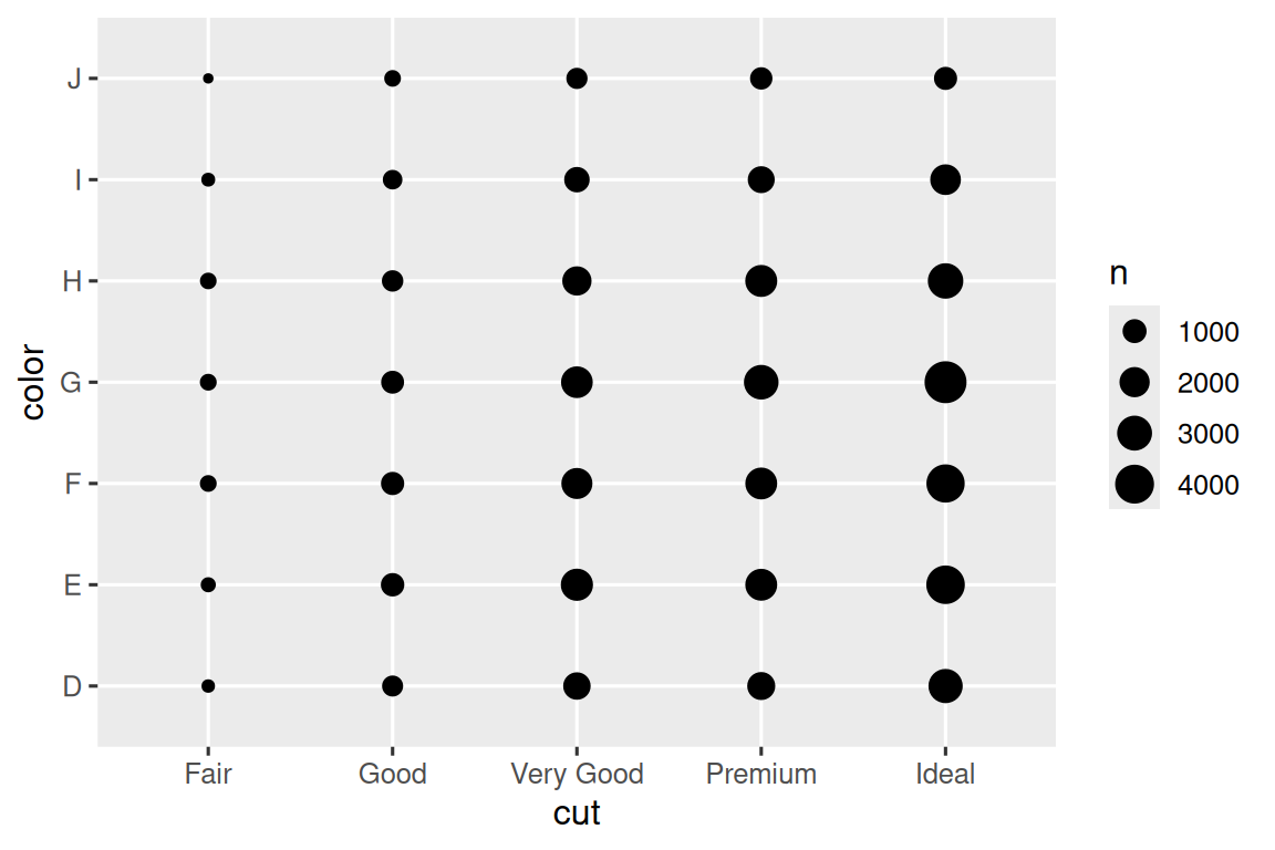

图中每个圆的大小显示在每个值组合下发生了多少观测。 协方差将显示为特定x值与特定y值之间的强相关性。

探索这些变量之间关系的另一种方法是使用 dplyr 计算计数（counts）：

diamonds |> 
  count(color, cut)
#> # A tibble: 35 × 3
#>   color cut           n
#>   <ord> <ord>     <int>
#> 1 D     Fair        163
#> 2 D     Good        662
#> 3 D     Very Good  1513
#> 4 D     Premium    1603
#> 5 D     Ideal      2834
#> 6 E     Fair        224
#> # ℹ 29 more rows

然后用 geom_tile() 和 fill aesthetic 可视化：

diamonds |> 
  count(color, cut) |>  
  ggplot(aes(x = color, y = cut)) +
  geom_tile(aes(fill = n))

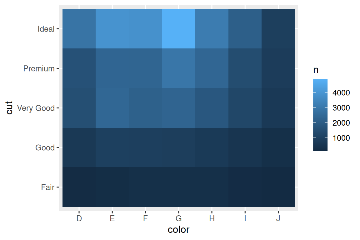
如果分类变量是无序的，则可能需要使用seriation软件包同时重新排序行（rows）和列（columns），以便更清楚地揭示有趣的模式。 对于较大的图，您可能需要尝试使用heatmaply软件包，从而创建交互式图。

10.5.2.1 Exercises

1. 您如何重新列出上述计数数据集以更清楚地显示color内cut的分布或cut中的color？

2. 如果将color映射到x美学并将cut映射到fill美学，则可以通过分段条形图获得哪些不同的数据见解？ 计算落入每个片段的计数。

3. 将geom_tile()与dplyr一起使用，以探索平均航班延误如何因目的地和一年的月份而异。 是什么使绘图难以阅读？ 你怎么能改善它？

10.5.3 Two numerical variables

您已经看到了一种可视化两个数值变量之间的协方差的好方法：用geom_point()绘制散点图。 您可以将协方差视为散点中的一种模式。 例如，您可以看到钻石的克拉尺寸（carat）和价格（price）之间的正相关关系：具有更大克拉尺寸（carat）的钻石价格（price）更高。 关系是指数级的。

ggplot(smaller, aes(x = carat, y = price)) +
  geom_point()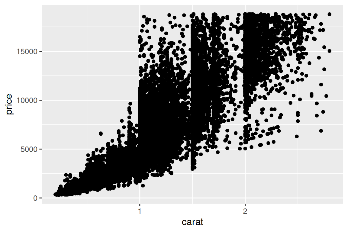

（在本节中，我们将使用smaller数据集专注于小于3克拉（carats）的大部分钻石）

随着数据集的大小的增长，散点图（Scatterplots）变得不那么有用，因为散点开始覆盖，并堆积成黑色均匀的区域，因此很难判断二维空间中数据密度的差异，并且很难发现趋势。 您已经看到了解决该问题的一种方法：使用 alpha aesthetic 添加透明度。

ggplot(smaller, aes(x = carat, y = price)) + 
  geom_point(alpha = 1 / 100)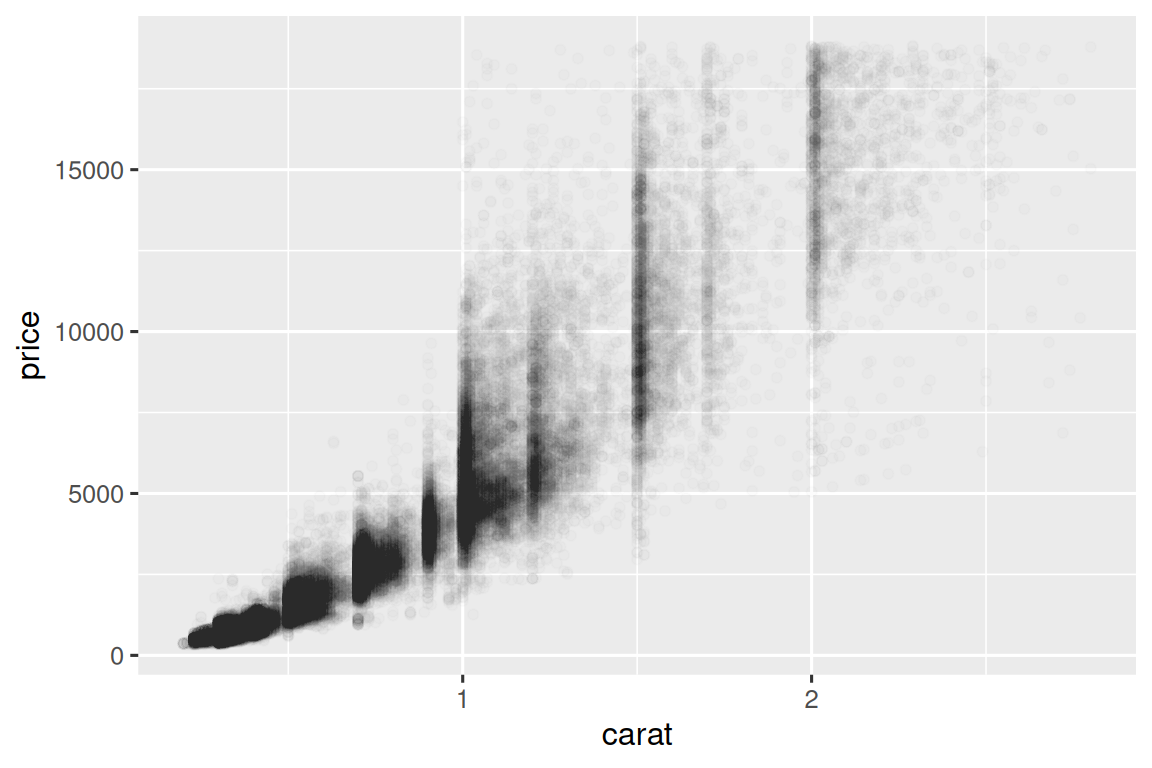

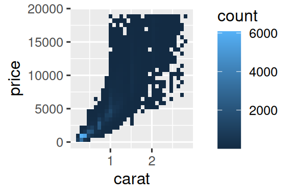
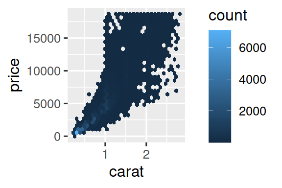
但是，对于非常大的数据集来说，使用透明度可能具有挑战性。 另一个解决方案是使用 bin。 以前，您使用 geom_histogram() 和 geom_freqpoly() 在一个维度上分 bin。 现在，您将学习如何使用 geom_bin2d() 和 geom_hex() 在二维中分 bin。

geom_bin2d() 和 geom_hex() 将坐标平面划分为 2d bins，然后使用 fill 颜色显示每个 bin 中落入多少点。 geom_bin2d() 创建矩形 bins。 geom_hex() 创建六角形 bins。 您将需要安装 hexbin 软件包以使用 geom_hex()。

ggplot(smaller, aes(x = carat, y = price)) +
  geom_bin2d()

# install.packages("hexbin")
ggplot(smaller, aes(x = carat, y = price)) +
  geom_hex()

另一个选择是对一个连续变量分 bin，以便它像一个分类变量。 然后，您可以使用其中一种技术来可视化您所学到的分类和连续变量的组合。 例如，您可以对 carat 分 bin，然后对于每个 group，显示一个箱形图：

ggplot(smaller, aes(x = carat, y = price)) + 
  geom_boxplot(aes(group = cut_width(carat, 0.1)))

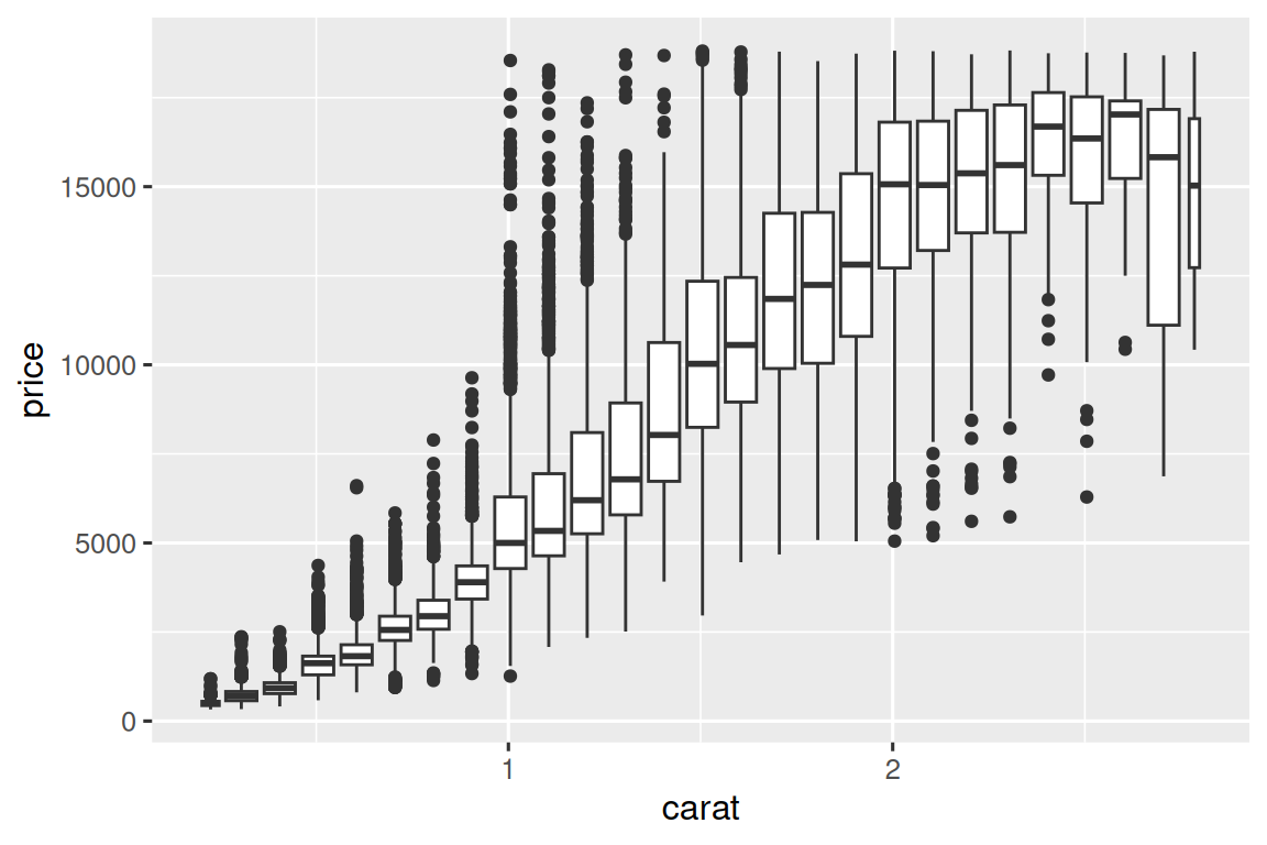
如上所述，cut_width(x, width) 将 x 分为宽度为 width 的 bins。 默认情况下，无论有多少观察值，箱线图看起来大致相同（除了数量的异常值），因此很难说每个箱线图总结了不同数量的点。 一种显示的方法是使箱线图的宽度与varwidth = TRUE的点数成比例。

10.5.3.1 Exercises

1. 您可以使用频率多边形，而不是用 boxplot 总结条件分布。 使用 cut_width() vs. cut_number() 时需要考虑什么？ 这如何影响 carat 和 price 的 2d 分布的可视化？

2. 可视化 carat 的分布，按 price 划分。

3. 非常大的钻石的价格分布与小钻石相比如何？ 是您所期望的，还是让您感到惊讶？

4. 结合您学会的两种技术来可视化 cut，carat 和 price 的组合分布。

5. 二维图揭示了在一维图中不可见的离群值。 例如，以下图中的某些点具有 x 和 y 值的异常组合，即使在单独检查时它们的 x 和 y 值显得正常，也使得散点异常。 为什么在这种情况下，scatterplot 比 binned plot 更好？

   diamonds |> 
     filter(x >= 4) |> 
     ggplot(aes(x = x, y = y)) +
     geom_point() +
     coord_cartesian(xlim = c(4, 11), ylim = c(4, 11))

6. 我们可以创建包含 cut_width() 大约相等数量的点的箱线图，而不是使用 cut_number() 创建相等宽度的箱线图。 这种方法的优点和缺点是什么？

   ggplot(smaller, aes(x = carat, y = price)) + 
     geom_boxplot(aes(group = cut_number(carat, 20)))

10.6 Patterns and models

如果两个变量之间存在系统关系，则将以数据模式出现。 如果您发现模式，请问自己：

• 这种模式可能是偶然的（即随机机会）吗？

• 您如何描述模式隐含的关系？

• 模式暗示的关系有多牢固？

• 其他哪些变量可能会影响这种关系？

• 如果您查看数据的各个子组，关系会改变吗？

数据中的模式提供了有关关系的线索，即它们揭示了协方差。 如果您将变化视为产生不确定性的现象，那么协方差是一种减少它的现象。 如果两个变量共变化，您可以使用一个变量的值来更好地预测第二个变量的值。 如果协方差是由于因果关系（特殊情况）引起的，则可以使用一个变量的值来控制第二个的值。

模型（Models）是从数据中提取模式的工具。 例如，考虑 diamonds 数据。 很难理解 cut 与 price 之间的关系，因为 cut 和 carat，以及 carat 和 price 密切相关。 可以使用模型来消除 price 和 carat 之间非常牢固的关系，因此我们可以探索剩下的微妙之处。 以下代码拟合一个模型，该模型可以从 carat 预测 price，然后计算残差（预测值和实际值之间的差异）。 一旦去除了 carat 的效果，残差使我们对钻石的 price 有所了解。 请注意，我们不使用 price 和 carat 的原始值，而是首先对其进行对数转换，并将模型拟合到对数转换值。 然后，我们指出残差以使它们的原始价格规模恢复。

library(tidymodels)

diamonds <- diamonds |>
  mutate(
    log_price = log(price),
    log_carat = log(carat)
  )

diamonds_fit <- linear_reg() |>
  fit(log_price ~ log_carat, data = diamonds)

diamonds_aug <- augment(diamonds_fit, new_data = diamonds) |>
  mutate(.resid = exp(.resid))

ggplot(diamonds_aug, aes(x = carat, y = .resid)) + 
  geom_point()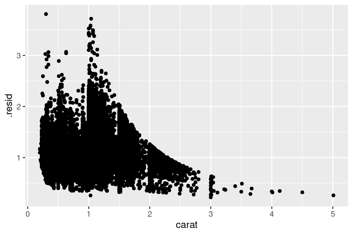

一旦你删除了 carat 和 price 之间的牢固关系后，您就可以看到 cut 与 price 之间的关系的期望：相对于它们的尺寸，质量更好的钻石更加昂贵。

ggplot(diamonds_aug, aes(x = cut, y = .resid)) + 
  geom_boxplot()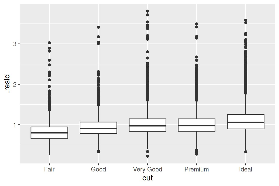

我们不在本书中讨论建模，因为一旦您拥有数据整理和编程工具，了解什么模型以及它们的工作方式最容易。

10.7 Summary

在本章中，您学到了各种工具，可以帮助您了解数据中的变化。 您已经看到了一次与单个变量一起使用的技术，并带有一对变量。 如果您的数据中有数十或数百个变量，这似乎是痛苦的限制，但是它们是所有其他技术的基础。

在下一章中，我们将重点介绍可以用来传达结果的工具。

---

1. 请记住，当我们需要明确函数（或数据集）来自何处时，我们将使用特殊形式 package::function() 或 package::dataset。