17 Dates and times
17.1 Introduction
本章将向你展示如何在 R 中处理日期和时间。 乍看之下,日期和时间似乎很简单。 你在日常生活中经常使用它们,而且它们似乎不会引起太多困惑。 然而,你对日期和时间了解得越多,就越会发现它们的复杂之处!
先来思考一下:一年有多少天,一天有多少小时。 你或许记得大多数年份有 365 天,但闰年有 366 天。 你知道判断闰年的完整规则吗1? 一天的小时数则稍不明显:大多数日子有 24 小时,但在使用夏令时(DST)的地区,每年会有一天只有 23 小时,另一天则有 25 小时。
日期和时间之所以复杂,是因为它们必须协调两种自然现象(地球自转和绕太阳公转)与一系列地缘政治现象(包括月份、时区和夏令时)。 本章不会涵盖日期和时间的每一个细节,但会为你打下扎实的实践技能基础,帮助你应对常见的数据分析挑战。
我们将首先展示如何从不同输入创建日期时间,然后介绍在获得日期时间后如何提取年、月、日等组成部分。 接着,我们将深入探讨处理时间跨度的棘手主题,根据不同的使用目标,时间跨度有多种表现形式。 最后,我们将简要讨论时区带来的额外挑战。
17.1.1 Prerequisites
本章将重点介绍 lubridate 包,它能让你在 R 中更轻松地处理日期和时间。 根据 tidyverse 的最新版本,lubridate 已成为核心 tidyverse 的一部分。 我们还需要 nycflights13 包来提供练习数据。
17.2 Creating date/times
有三种类型的日期/时间数据用于指代特定时刻:
A date。 Tibbles 会将其显示为
<date>。A time within a day。 Tibbles 会将其显示为
<time>。A date-time 是日期加上时间: 它能唯一标识某个时刻(通常精确到秒)。 Tibbles 会将其显示为
<dttm>。 Base R 将其称为 POSIXct, 但这个名称并不直观.
本章我们将重点关注日期和日期时间,因为 R 没有原生类来存储时间。 如果你需要处理时间,可以使用 hms 包。
你应始终使用能满足需求的最简单数据类型。 这意味着如果可以用 date 代替 date-time,就应该使用 date。 Date-times 要复杂得多,因为需要处理时区问题,我们将在本章末尾讨论这一点。
要获取当前 date 或 date-time,可以使用 today() 或 now():
除此之外,以下部分将介绍四种常见的创建 date/time 的方法:
- 使用 readr 读取文件时。
- 从字符串解析。
- 从独立的 date-time 组件组合。
- 从已有的 date/time 对象转换。
17.2.1 During import
如果你的 CSV 文件包含 ISO8601 格式的 date 或 date-time,你无需进行额外操作;readr 会自动识别它:
csv <- "
  date,datetime
  2022-01-02,2022-01-02 05:12
"
read_csv(csv)
#> Warning: The `file` argument of `read_csv()` should use `I()` for literal data as of
#> readr 2.2.0.
#>
#>   # Bad (for example):
#>   read_csv("x,y\n1,2")
#>
#>   # Good:
#>   read_csv(I("x,y\n1,2"))
#> # A tibble: 1 × 2
#>   date       datetime
#>   <date>     <dttm>
#> 1 2022-01-02 2022-01-02 05:12:00
如果你之前没听说过 ISO8601,它是一种国际标准2,用于书写日期,其日期组成部分按从大到小的顺序排列,并用 - 分隔。 例如,在 ISO8601 标准中,2022 年 5 月 3 日写作 2022-05-03。ISO8601 日期也可以包含时间,其中时、分、秒用 : 分隔,而日期和时间部分则用 T 或空格分隔。 例如,2022 年 5 月 3 日下午 4:26 可以写作 2022-05-03 16:26 或 2022-05-03T16:26。
对于其他日期时间格式,你需要使用 col_types 以及 col_date() 或 col_datetime(),并指定日期时间格式。 readr 使用的日期时间格式是多种编程语言通用的标准,它用 % 后跟一个字符来描述日期组成部分。 例如,%Y-%m-%d 指定了一个日期格式为年、-、月(数字形式)、-、日。 表 Table 17.1 列出了所有选项。
| Type | Code | Meaning | Example |
|---|---|---|---|
| Year | %Y |
4 digit year | 2021 |
%y |
2 digit year | 21 | |
| Month | %m |
Number | 2 |
%b |
Abbreviated name | Feb | |
%B |
Full name | February | |
| Day | %d |
Two digits | 02 |
%e |
One or two digits | 2 | |
| Time | %H |
24-hour hour | 13 |
%I |
12-hour hour | 1 | |
%p |
AM/PM | pm | |
%M |
Minutes | 35 | |
%S |
Seconds | 45 | |
%OS |
Seconds with decimal component | 45.35 | |
%Z |
Time zone name | America/Chicago | |
%z |
Offset from UTC | +0800 | |
| Other | %. |
Skip one non-digit | : |
%* |
Skip any number of non-digits |
这段代码显示了一些应用于一个非常模糊的日期的选项:
csv <- "
  date
  01/02/15
"

read_csv(csv, col_types = cols(date = col_date("%m/%d/%y")))
#> # A tibble: 1 × 1
#>   date
#>   <date>
#> 1 2015-01-02

read_csv(csv, col_types = cols(date = col_date("%d/%m/%y")))
#> # A tibble: 1 × 1
#>   date
#>   <date>
#> 1 2015-02-01

read_csv(csv, col_types = cols(date = col_date("%y/%m/%d")))
#> # A tibble: 1 × 1
#>   date
#>   <date>
#> 1 2001-02-15
请注意,无论你如何指定日期格式,一旦将其导入 R,它总是以相同的方式显示。
如果你使用 %b 或 %B 并处理非英语日期,还需要提供 locale() 参数。 可查看 date_names_langs() 中内置的语言列表,或使用 date_names() 创建自定义语言设置。
17.2.2 From strings
日期时间规范语言功能强大,但需要仔细分析日期格式。 另一种方法是使用 lubridate 的辅助函数,它们能在你指定组成部分的顺序后自动判断格式。 使用时,只需识别你的日期中年、月、日出现的顺序,然后按相同顺序排列 “y”、“m” 和 “d”。 即可得到能解析该日期的 lubridate 函数名称。 例如:
ymd() 等创建 data。 要创建 date-time,请在解析函数的名称中添加下划线和一个或多个 “h”,“m” 和 “s”:
你也可以通过提供时区来强制从 date 创建 date-time:
ymd("2017-01-31", tz = "UTC")
#> [1] "2017-01-31 UTC"
这里我使用了 UTC3 时区,你可能也知道它被称为 GMT(格林威治标准时间),即经度 0° 的时间4 。该时区不采用夏令时,这使得计算更为简便 。
17.2.3 From individual components
有时,你会遇到 date-time 的各个组成部分分散在多个列中,而不是单个字符串。 flights 数据集中的情况正是如此:
flights |>
  select(year, month, day, hour, minute)
#> # A tibble: 336,776 × 5
#>    year month   day  hour minute
#>   <int> <int> <int> <dbl>  <dbl>
#> 1  2013     1     1     5     15
#> 2  2013     1     1     5     29
#> 3  2013     1     1     5     40
#> 4  2013     1     1     5     45
#> 5  2013     1     1     6      0
#> 6  2013     1     1     5     58
#> # ℹ 336,770 more rows
要从这类输入创建 date/time,请对 dates 使用 make_date(),对 date-times 使用 make_datetime():
flights |>
  select(year, month, day, hour, minute) |>
  mutate(departure = make_datetime(year, month, day, hour, minute))
#> # A tibble: 336,776 × 6
#>    year month   day  hour minute departure
#>   <int> <int> <int> <dbl>  <dbl> <dttm>
#> 1  2013     1     1     5     15 2013-01-01 05:15:00
#> 2  2013     1     1     5     29 2013-01-01 05:29:00
#> 3  2013     1     1     5     40 2013-01-01 05:40:00
#> 4  2013     1     1     5     45 2013-01-01 05:45:00
#> 5  2013     1     1     6      0 2013-01-01 06:00:00
#> 6  2013     1     1     5     58 2013-01-01 05:58:00
#> # ℹ 336,770 more rows
让我们对 flights 中的四个时间列进行同样的处理。 时间的表示格式有些特殊,因此我们使用模运算来提取小时和分钟部分。 创建 date-time 变量后,我们将重点关注本章后续部分要探索的变量。
make_datetime_100 <- function(year, month, day, time) {
  make_datetime(year, month, day, time %/% 100, time %% 100)
}

flights_dt <- flights |>
  filter(!is.na(dep_time), !is.na(arr_time)) |>
  mutate(
    dep_time = make_datetime_100(year, month, day, dep_time),
    arr_time = make_datetime_100(year, month, day, arr_time),
    sched_dep_time = make_datetime_100(year, month, day, sched_dep_time),
    sched_arr_time = make_datetime_100(year, month, day, sched_arr_time)
  ) |>
  select(origin, dest, ends_with("delay"), ends_with("time"))

flights_dt
#> # A tibble: 328,063 × 9
#>   origin dest  dep_delay arr_delay dep_time            sched_dep_time
#>   <chr>  <chr>     <dbl>     <dbl> <dttm>              <dttm>
#> 1 EWR    IAH           2        11 2013-01-01 05:17:00 2013-01-01 05:15:00
#> 2 LGA    IAH           4        20 2013-01-01 05:33:00 2013-01-01 05:29:00
#> 3 JFK    MIA           2        33 2013-01-01 05:42:00 2013-01-01 05:40:00
#> 4 JFK    BQN          -1       -18 2013-01-01 05:44:00 2013-01-01 05:45:00
#> 5 LGA    ATL          -6       -25 2013-01-01 05:54:00 2013-01-01 06:00:00
#> 6 EWR    ORD          -4        12 2013-01-01 05:54:00 2013-01-01 05:58:00
#> # ℹ 328,057 more rows
#> # ℹ 3 more variables: arr_time <dttm>, sched_arr_time <dttm>, …
利用这些数据,我们可以可视化一年中起飞时间的分布情况:
flights_dt |>
  ggplot(aes(x = dep_time)) +
  geom_freqpoly(binwidth = 86400) # 86400 seconds = 1 day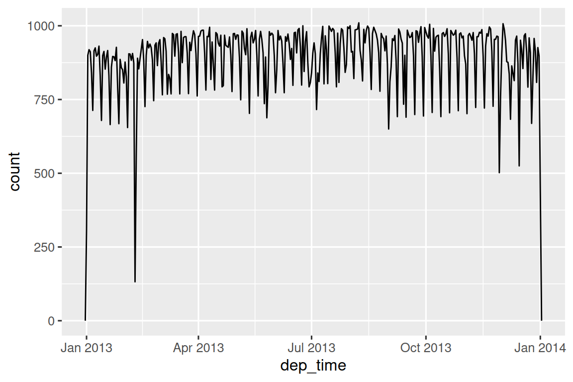
或者在一天之内:
flights_dt |>
  filter(dep_time < ymd(20130102)) |>
  ggplot(aes(x = dep_time)) +
  geom_freqpoly(binwidth = 600) # 600 s = 10 minutes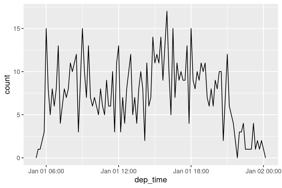
请注意,当您在数字上下文中(如直方图中)使用 date-times 时,1 表示 1 秒,因此 binwidth 为 86400 表示一天。 对于 dates,1 表示 1 天。
17.2.4 From other types
你可能需要在 date-time 和 date 之间进行转换。 这可以通过 as_datetime() 和 as_date() 函数来实现:
as_datetime(today())
#> [1] "2026-06-15 UTC"
as_date(now())
#> [1] "2026-06-15"
有时你会遇到以数字偏移量形式表示的 date/times,其基准是 “Unix Epoch”,1970-01-01。 如果偏移量以秒为单位,请使用 as_datetime();如果以天为单位,则使用 as_date()。
as_datetime(60 * 60 * 10)
#> [1] "1970-01-01 10:00:00 UTC"
as_date(365 * 10 + 2)
#> [1] "1980-01-01"
17.2.5 Exercises
17.3 Date-time components
现在你已经知道如何将 date-time 数据导入 R 的 date-time 数据结构,接下来让我们探索可以对它们进行哪些操作。 本节将重点介绍用于获取和设置单个组件的访问器函数。 下一节将探讨 date-times 的算术运算。
17.3.1 Getting components
你可以使用访问器函数 year(), month(), mday() (day of the month), yday() (day of the year), wday() (day of the week), hour(), minute(), 和 second() 来提取日期的各个组成部分。 这些函数实际上是 make_datetime() 的反向操作。
对于 month() 和 wday() 函数,你可以设置 label = TRUE 来返回月份或星期几的缩写名称。 设置 abbr = FALSE 可返回完整名称。
我们可以使用 wday() 来观察工作日出发的航班数量多于周末:

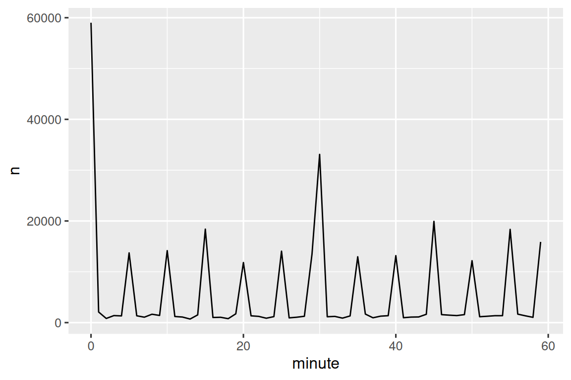
我们还可以观察每小时之内分钟粒度的平均起飞延误情况。 这里有一个有趣的规律:在 20-30 分钟和 50-60 分钟起飞的航班,其延误程度远低于该小时内其他时段的航班!
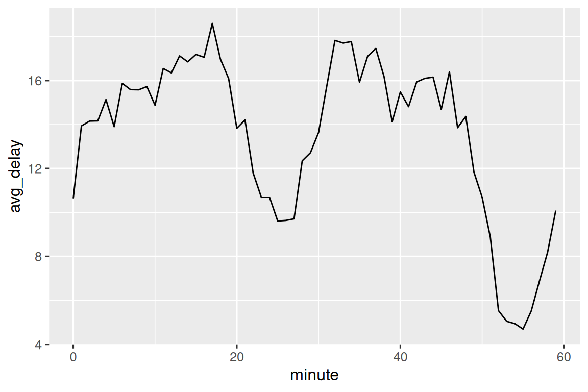
有趣的是,如果我们查看计划起飞时间,并没有观察到如此明显的规律:
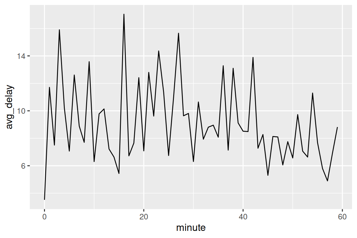
那么,为什么在实际起飞时间中会出现这种规律呢? 事实上,如同许多由人工收集的数据一样,航班倾向于在“整点”时间起飞,如 Figure 17.1 所示,这导致了明显的偏差。 在处理涉及人为判断的数据时,务必警惕这类规律的存在!
17.3.2 Rounding
另一种绘制单个日期组成部分的方法是使用 floor_date()、round_date() 和 ceiling_date() 函数,将日期四舍五入到附近的时间单位。 每个函数都接受一个待调整的日期向量,以及要向下取整(floor)、向上取整(ceiling)或四舍五入(round)的时间单位名称。 例如,这使我们能够绘制每周的航班数量:
flights_dt |>
  count(week = floor_date(dep_time, "week")) |>
  ggplot(aes(x = week, y = n)) +
  geom_line() +
  geom_point()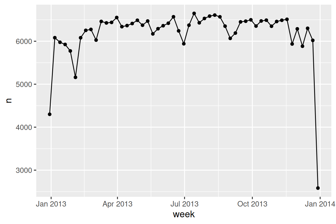
通过计算 dep_time 与当天最早时刻之间的差值,你可以使用四舍五入来展示航班在一天内的分布情况:
flights_dt |>
  mutate(dep_hour = dep_time - floor_date(dep_time, "day")) |>
  ggplot(aes(x = dep_hour)) +
  geom_freqpoly(binwidth = 60 * 30)
#> Don't know how to automatically pick scale for object of type <difftime>.
#> Defaulting to continuous.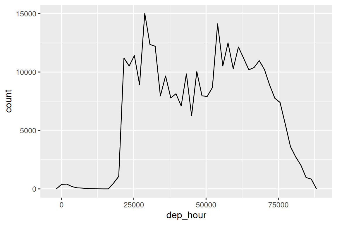
计算两个日期时间之间的差值会得到一个 difftime 对象(更多内容见 Section 17.4.3 节)。 我们可以将其转换为 hms 对象,以获得更有用的 x 轴:
flights_dt |>
  mutate(dep_hour = hms::as_hms(dep_time - floor_date(dep_time, "day"))) |>
  ggplot(aes(x = dep_hour)) +
  geom_freqpoly(binwidth = 60 * 30)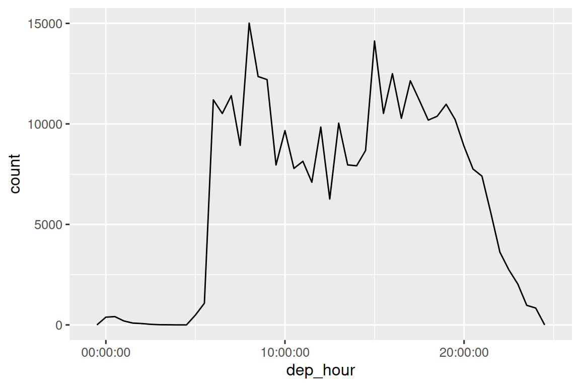
17.3.3 Modifying components
你也可以使用每个访问器函数来修改 date/time 的组成部分。 这在数据分析中不常用,但在清理日期明显错误的数据时可能很有用。
或者,你无需修改现有变量,而是可以使用 update() 创建一个新的 date-time。 这还允许你一步设置多个值:
update(datetime, year = 2030, month = 2, mday = 2, hour = 2)
#> [1] "2030-02-02 02:34:56 UTC"
如果设置的值过大,它们会自动向前进位:
17.3.4 Exercises
一天内航班时间的分布如何随一年中的时间变化?
比较
dep_time,sched_dep_time和dep_delay。 它们是否一致? 请解释你的发现。比较
air_time与起飞和到达之间的时间间隔。 解释你的发现。 (提示:考虑机场的位置。)一天中平均延误时间如何变化? 应该使用
dep_time还是sched_dep_time? 为什么?如果希望最小化延误的可能性,你应该在一周中的哪一天出发?
diamonds$carat和flights$sched_dep_time的分布有何相似之处?验证我们的假设:20-30 分钟和 50-60 分钟起飞的航班较早出发是由于计划航班提前起飞所致。 提示:创建一个二元变量来指示航班是否延误。
17.4 Time spans
接下来,你将学习日期算术运算的原理,包括减法、加法和除法。 在此过程中,你会了解到三种表示时间跨度的重要类别:
- Durations, 表示精确的秒数。
- Periods, 表示人类可理解的单位,如周 (weeks) 和月 (months)。
- Intervals, 表示一个起始点和结束点。
如何在 duration、periods 和 intervals 之间做出选择? 一如既往,选择能解决你问题的最简单数据结构。 如果你只关心物理时间,使用 duration;如果需要添加人类可理解的时间,使用 period;如果需要计算某个跨度在人类单位中的长度,使用 interval。
17.4.1 Durations
在 R 中,当你对两个日期进行相减时,会得到一个 difftime 对象:
difftime 类对象以秒、分钟、小时、天或周为单位记录时间跨度。 这种模糊性可能使得 difftimes 对象处理起来有些棘手,因此 lubridate 提供了另一种始终以秒为单位的时间跨度表示方式:duration。
as.duration(h_age)
#> [1] "1472774400s (~46.67 years)"
Durations 附带了一系列便捷的构造函数:
dseconds(15)
#> [1] "15s"
dminutes(10)
#> [1] "600s (~10 minutes)"
dhours(c(12, 24))
#> [1] "43200s (~12 hours)" "86400s (~1 days)"
ddays(0:5)
#> [1] "0s"                "86400s (~1 days)"  "172800s (~2 days)"
#> [4] "259200s (~3 days)" "345600s (~4 days)" "432000s (~5 days)"
dweeks(3)
#> [1] "1814400s (~3 weeks)"
dyears(1)
#> [1] "31557600s (~1 years)"
Durations 始终以秒为单位记录时间跨度。 更大的单位通过将分钟、小时、天、周和年转换为秒来创建:一分钟 60 秒,一小时 60 分钟,一天 24 小时,一周 7 天。 更大的时间单位则更具问题性。 一年使用“平均”年天数,即 365.25 天。 由于月份的变化太大,无法将其转换为 duration。
你可以对 durations 进行加减和乘法运算:
你可以对日期进行 durations 的加减运算:
然而,由于 durations 表示的是精确的秒数,有时你可能会得到意想不到的结果:
为什么 3 月 8 日凌晨 1 点加上一天后是 3 月 9 日凌晨 2 点? 如果仔细观察日期,你可能还会注意到时区发生了变化。 3 月 8 日只有 23 小时,因为这是夏令时开始的时间,所以如果我们加上一整天的秒数,最终会得到一个不同的时间。
17.4.2 Periods
为了解决这个问题,lubridate 提供了 periods。 Periods 表示时间跨度,但其长度不以固定的秒数为单位,而是以“人类”时间(如 days 和 months)为单位。 这使得它们能以更直观的方式工作:
one_am
#> [1] "2026-03-08 01:00:00 EST"
one_am + days(1)
#> [1] "2026-03-09 01:00:00 EDT"
与 durations 类似,periods 也可以通过一系列便捷的构造函数来创建。
你可以对 periods 进行加法和乘法运算:
当然,也可以将它们与 dates 相加。 与 durations 相比,periods 更可能符合你的预期:
让我们使用 periods 来解决与航班日期相关的一个异常情况。 一些飞机似乎在其从纽约市起飞之前就已到达目的地。
flights_dt |>
  filter(arr_time < dep_time)
#> # A tibble: 10,633 × 9
#>   origin dest  dep_delay arr_delay dep_time            sched_dep_time
#>   <chr>  <chr>     <dbl>     <dbl> <dttm>              <dttm>
#> 1 EWR    BQN           9        -4 2013-01-01 19:29:00 2013-01-01 19:20:00
#> 2 JFK    DFW          59        NA 2013-01-01 19:39:00 2013-01-01 18:40:00
#> 3 EWR    TPA          -2         9 2013-01-01 20:58:00 2013-01-01 21:00:00
#> 4 EWR    SJU          -6       -12 2013-01-01 21:02:00 2013-01-01 21:08:00
#> 5 EWR    SFO          11       -14 2013-01-01 21:08:00 2013-01-01 20:57:00
#> 6 LGA    FLL         -10        -2 2013-01-01 21:20:00 2013-01-01 21:30:00
#> # ℹ 10,627 more rows
#> # ℹ 3 more variables: arr_time <dttm>, sched_arr_time <dttm>, …
这些是过夜航班。 我们在起飞和到达时间中使用了相同的日期信息,但这些航班实际上是在第二天抵达的。 我们可以通过为每个过夜航班的到达时间加上 days(1) 来修正这个问题。
现在,所有航班都符合物理定律了。
flights_dt |>
  filter(arr_time < dep_time)
#> # A tibble: 0 × 10
#> # ℹ 10 variables: origin <chr>, dest <chr>, dep_delay <dbl>,
#> #   arr_delay <dbl>, dep_time <dttm>, sched_dep_time <dttm>, …
17.4.3 Intervals
dyears(1) / ddays(365) 会返回什么结果? 它并不完全等于 1,因为 dyears() 被定义为每个平均年份的秒数,即 365.25 天。
那么 years(1) / days(1) 会返回什么? 如果年份是 2015,它应该返回 365;但如果是 2016,它应该返回 366! lubridate 没有足够的信息来给出一个唯一明确的答案。 它实际做的是给出一个估算值:
如果你想要更精确的测量,就必须使用 interval。 interval 是一对起始和结束的日期时间,或者你可以将其视为带有起始点的时长。
你可以通过 start %--% end 的语法创建一个区间:
然后你可以将其除以 days() 来找出该年份包含多少天:
17.4.4 Exercises
向刚学习 R 的人解释
days(!overnight)和days(overnight)。 你需要了解的关键事实是什么?创建一个日期向量,表示 2015 年每个月的第一天。 再创建一个日期向量,表示当前年份每个月的第一天。
编写一个函数,根据你的生日(作为日期输入),返回你的年龄(以年为单位)。
为什么
(today() %--% (today() + years(1))) / months(1)无法运行?
17.5 Time zones
时区是一个极其复杂的主题,因为它们与地缘政治实体相互作用。 幸运的是,我们不需要深入探究所有细节,因为并非所有细节对数据分析都至关重要,但有一些挑战我们确实需要直面应对。
第一个挑战是日常使用的时区名称往往具有歧义性。 例如,如果你是美国人,可能很熟悉 EST(东部标准时间)。 然而,澳大利亚和加拿大也都有 EST! 为了避免混淆,R 采用国际标准的 IANA 时区。 这些时区使用一致的命名规则 {area}/{location},通常形式为 {continent}/{city} 或 {ocean}/{city}。 例如:“America/New_York”、“Europe/Paris” 和 “Pacific/Auckland”。
你可能会好奇,为什么时区使用城市名称,而通常我们认为时区与国家或国家内的区域相关联。 这是因为 IANA 数据库必须记录数十年的时区规则。 在几十年间,国家名称变更(或分裂)相当频繁,但城市名称往往保持不变。 另一个问题是,名称不仅需要反映当前行为,还需体现完整的历史。 例如,同时存在 “America/New_York” 和 “America/Detroit” 两个时区。 这两个城市目前都使用东部标准时间,但在 1969-1972 年间,密歇根州(底特律所在州)未遵循夏令时,因此需要一个不同的名称。 值得一读原始时区数据库(可在 https://www.iana.org/time-zones 获取),仅是为了了解其中的一些历史故事!
你可以通过 Sys.timezone() 查看 R 认为你当前的时区是什么:
Sys.timezone()
#> [1] "UTC"
(如果 R 无法识别,则会返回 NA。)
可以通过 OlsonNames() 查看完整的时区名称列表:
length(OlsonNames())
#> [1] 598
head(OlsonNames())
#> [1] "Africa/Abidjan"     "Africa/Accra"       "Africa/Addis_Ababa"
#> [4] "Africa/Algiers"     "Africa/Asmara"      "Africa/Asmera"
在 R 中,时区是 date-time 的一个属性,仅控制显示方式。 例如,以下三个对象表示同一时刻:
你可以通过减法运算验证它们是同一时间:
x1 - x2
#> Time difference of 0 secs
x1 - x3
#> Time difference of 0 secs
除非另有说明,lubridate 始终使用 UTC。 UTC(协调世界时)是科学界使用的标准时区,大致等同于 GMT(格林威治标准时间)。 它不采用夏令时,因此便于计算。 组合 date-times 的操作(如 c())通常会丢弃时区信息。 这种情况下,date-times 将按第一个元素的时区显示:
x4 <- c(x1, x2, x3)
x4
#> [1] "2024-06-01 12:00:00 EDT" "2024-06-01 12:00:00 EDT"
#> [3] "2024-06-01 12:00:00 EDT"
你可以通过两种方式更改时区:
-
保持时间点不变,仅改变其显示方式。 当时间点正确但希望以更自然的方式显示时使用此方法。
x4a <- with_tz(x4, tzone = "Australia/Lord_Howe")
x4a
#> [1] "2024-06-02 02:30:00 +1030" "2024-06-02 02:30:00 +1030"
#> [3] "2024-06-02 02:30:00 +1030"
x4a - x4
#> Time differences in secs
#> [1] 0 0 0
(这也说明了时区的另一个挑战:它们并非都是整小时的偏移量!)
-
改变底层的时间点。 当时间点被标记了错误的时区且需要修正时使用此方法。
x4b <- force_tz(x4, tzone = "Australia/Lord_Howe")
x4b
#> [1] "2024-06-01 12:00:00 +1030" "2024-06-01 12:00:00 +1030"
#> [3] "2024-06-01 12:00:00 +1030"
x4b - x4
#> Time differences in hours
#> [1] -14.5 -14.5 -14.5
17.6 Summary
本章向你介绍了 lubridate 提供的工具,帮助你处理日期时间数据。 处理日期和时间看似比实际需要的更复杂,但希望本章能让你理解其原因——日期时间比乍看之下更为复杂,而处理各种可能的情况增加了其复杂性。 即使你的数据从未涉及夏令时变更或闰年,相关函数也必须能够应对这些情况。
下一章将系统总结缺失值的处理方法。 你已经在多个场景中遇到过缺失值,在自己的分析中也无疑会碰到它们。现 在,是时候提供一个实用技巧合集来应对这些情况了。